In mid-March 2024, as the price of Bitcoin repeatedly set new record highs, open interest in the derivatives market briefly approached a peak of nearly $38 billion, after which a price pullback of just 7% triggered more than $800 million in cascading liquidations [1]. This episode highlights a core structural feature of the crypto-asset derivatives market: the eruption of systemic risk often stems not from a fundamental reversal in price direction but from a nonlinear expansion of volatility over an extremely short interval. For market participants, understanding the sources and clustering mechanisms of volatility is only the first step; the more challenging question is how to translate this theoretical understanding into executable forecasting models and risk-control decisions. That question is the central analytical objective of this chapter.
A market maker need not forecast the direction of Bitcoin's next-day price move, but must estimate its next-day volatility accurately. When expected volatility rises, the rational response is to widen the quoted spread, reduce order book depth, and tighten inventory limits; when volatility is expected to stay low, the market maker can quote narrower spreads and provide deeper liquidity [2]. What the market maker forecasts, in short, is not direction but the dynamics of volatility. The same holds for a portfolio manager, for whom the precise level of returns matters far less than the width of the return distribution, because that width drives the calibration of value at risk (VaR) and the sizing of positions [3]. And for exchanges and protocol designers, guarding against systemic risk turns on predicting which level of volatility will push liquidation volume past safety thresholds, so that margin requirements can be raised preemptively [4].
Volatility forecasting cannot reveal the specific events that will occur, but it can quantify the magnitude of the impact that potential events would have on market prices. Chapter 22 established a framework decomposing volatility into four sources, and Chapter 23 analyzed the clustering and regime-switching of volatility; the task of this chapter is to build, on that foundation, a set of operational forecasting models and a decision-making system. Classical volatility-clustering theory holds that large price changes tend to be followed by further large changes [5], an empirical regularity widely verified in traditional financial markets. The crypto-asset perpetual futures market, however, has distinctive properties—24/7 continuous trading, periodic funding settlement, and the absence of a deep options market—that call for targeted structural adjustments to the classical generalized autoregressive conditional heteroskedasticity (GARCH) model and the heterogeneous autoregressive (HAR) model [6].
This chapter begins with the volatility information set specific to the perpetual futures market and examines the predictive power of the funding rate, liquidation heatmaps, and order book shape in the absence of implied volatility. On that basis, it proposes a source-decomposed volatility forecasting framework that models informational, liquidity, mechanical, and transmission volatility separately before aggregating them, precisely because these sources differ so fundamentally in predictability and time scale. Those forecasts are then embedded in a three-layer decision architecture spanning micro-level market-making quotes, meso-level position management, and macro-level systemic defenses. By the end of the chapter, the reader should be able to judge where different volatility-forecasting models apply to perpetual futures data, use alternative signals to read the market's risk state, and locate the boundary between the modelable and the intrinsically unpredictable components of volatility—the knowledge on which more resilient trading and risk-control systems are built.
24.1 The set of alternative volatility signals for perpetual futures
In traditional financial markets, option-implied volatility provides participants with a unified, forward-looking volatility benchmark. In the cryptocurrency perpetual futures market, however, the vast majority of assets lack a deep options market. This structural gap forces participants to construct an alternative system of volatility signals from dimensions such as the funding rate, liquidation heatmaps, order book microstructure, and on-chain data. This section analyzes the information content and predictive power of these signals in turn, assessing the conditions under which each class applies across different time scales.
24.1.1 The absence of implied volatility
In traditional financial markets, the core input for volatility forecasting is the implied volatility supplied by the options market. The Chicago Board Options Exchange's VIX, a measure of the implied volatility of S&P 500 index options, is widely used as a benchmark for gauging market risk expectations and the level of volatility over the next 30 days [7]. The distinctive value of implied volatility lies in its forward-looking nature: it is not a simple extrapolation of historical price movements but a consensus price reached by market participants through actual option-trading positions. When market makers and institutional investors expect volatility to rise, they demand higher option premiums, which directly pushes up the implied-volatility measure.
Although the cryptocurrency market has developed a derivatives ecosystem of some scale, its structure differs markedly from that of traditional finance. Platforms such as Deribit offer options trading on Bitcoin and Ethereum and have launched a VIX-like index, the Deribit volatility index (DVOL) [8]; nonetheless, the depth, liquidity, and breadth of participation in crypto options markets remain far below those of traditional markets. More important, although platforms such as Deribit have extended options coverage to leading altcoins such as SOL and XRP, and decentralized options platforms such as Aevo offer a broader product line, most altcoins still lack options markets with sufficient depth and liquidity. As a result of this structural feature, perpetual futures participants cannot rely on a unified, deep implied-volatility indicator when making trading and risk-management decisions.
The absence of implied volatility has forced the perpetual futures ecosystem to develop a distinctive system of alternative signals. These signals are scattered across the funding rate, order book shape, liquidation data, and on-chain fund flows. Although no single signal can match the precision of the VIX, by cross-validating microstructure data across multiple dimensions, participants can still construct a highly informative set of volatility predictors. Figure 24-1 maps these six classes of volatility information source against the time scale over which each forecasts effectively and its relative predictive power, giving an overview of the volatility information available in the perpetual futures ecosystem.
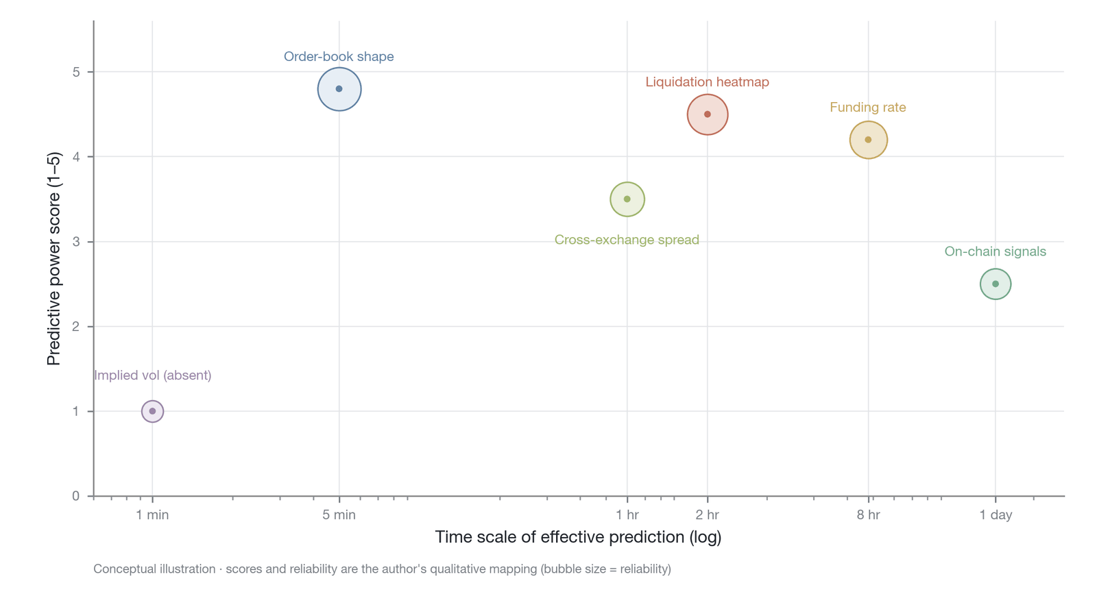
Figure 24-1. A panorama of the volatility information set for perpetual futures (conceptual mapping: the horizontal time-scale axis reflects true orders of magnitude, whereas the vertical predictive-power scores and the bubble reliability are the author's qualitative assignments rather than measured data; data source: compiled by the author)
The signals form a complementary gradient across time scales, running from minute-level order book shape to multi-day on-chain and cross-market signals. It is this layered, multi-scale structure that compensates for the missing implied-volatility benchmark: no single signal replaces the breadth of information in the VIX, but the six sources together yield useful forward-looking judgments within the windows where each is strongest. The subsections below take up the mechanism and predictive logic of each class in turn.
24.1.2 The funding rate as a volatility signal
The funding rate is the core mechanism in perpetual futures that regulates the balance of long and short positions and anchors the contract to the spot price (as discussed in Chapter 17) [9]. Beyond its own arbitrage value, its dynamics carry information for forecasting volatility. When the funding rate turns extreme—when its absolute value deviates sharply from baseline levels—it is often a reliable precursor to rising market volatility, because an extreme reading directly reflects a severe imbalance between long and short forces in the market.
The intrinsic link between extreme funding rates and rising volatility stems from a severe imbalance in directional demand. A very high positive rate indicates that longs dominate, with large amounts of leveraged capital chasing the uptrend; a deeply negative rate reflects extreme crowding on the short side. Such an imbalance is inherently fragile. When the market price moves in the opposite direction, the side bearing the high funding cost faces enormous pressure to close positions. This closing activity consumes liquidity on one side, which in turn amplifies price volatility. Extreme funding rates therefore not only reflect an excessive concentration of the market's current directional preference but also foreshadow potential future liquidation risk and volatility jumps.
Beyond the absolute level of the rate, the speed at which the funding rate changes—the volatility of the rate—is likewise a highly informative predictor. When the funding rate fluctuates violently over a short interval, especially when it flips rapidly from strongly positive to strongly negative, it signals that the market structure is undergoing an abrupt reorganization. This reorganization is accompanied by the opening and closing of large volumes of positions, which is itself a direct manifestation of a liquidity shock. Empirical observation indicates that the speed of funding-rate changes tends to correlate positively with realized volatility over the subsequent 1 to 24 hours, consistent with the rapid transmission of rate information under the cross-platform tiered structure of the crypto funding rate market [10]. Figure 24-2 illustrates how extreme funding rates and their rate of change predict short-term volatility, plotting subsequent realized volatility against the absolute level of the rate in one panel and against the speed of rate changes in the other.
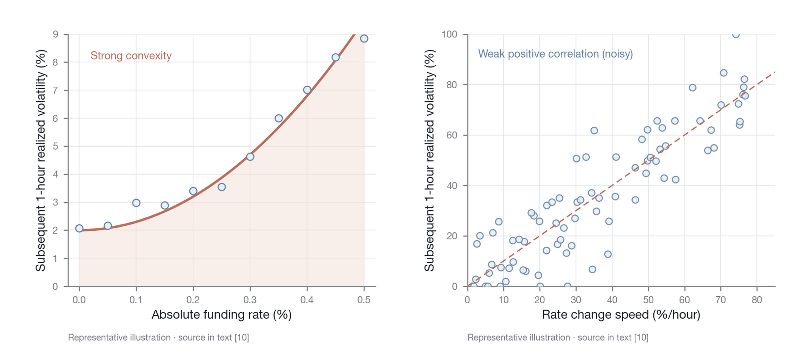
Figure 24-2. The predictive relationship between extreme funding rates and subsequent volatility (representative illustrative relationship: noisy scatter, not an empirical dataset; the tiered structure of the funding rate market follows Zhivkov 2026 [10])
The figure reveals two noteworthy patterns. When the absolute value of the funding rate exceeds two standard deviations above its historical mean, the probability of a marked jump in realized volatility over the subsequent 1 to 24 hours increases substantially; this threshold effect makes extreme funding rates an early-warning signal with a well-defined trigger condition. The speed of rate changes has independent predictive value as well: even when the absolute level of the rate has not yet reached the extreme zone, rapid changes in it reveal that the market microstructure is undergoing an abrupt adjustment. The combination of these two dimensions forms a two-dimensional rate-warning matrix, in which the "high absolute level plus rapid change" quadrant corresponds to the highest short-term volatility risk.
24.1.3 Liquidation heatmaps
A distinctive source of risk in the perpetual futures market is the cascade effect triggered by the automatic liquidation mechanism (as discussed in Chapter 22). A liquidation heatmap maps the liquidation prices of all current open positions onto specific price ranges, giving a direct view of the scale of liquidations latent at different price levels. This spatial distribution is essentially a map of volatility risk, providing a key microstructure clue for forecasting mechanical volatility [11].
The predictive logic of a liquidation heatmap rests on the spatial distance between the price and dense clusters of liquidations. If the current market price is only a very short distance from a cluster containing a large volume of liquidatable positions, and the expected liquidation volume in that zone far exceeds the absorptive capacity of the current order book, then once the price reaches that zone it will inevitably trigger a liquidation cascade. In such a scenario, the liquidation engine dumps a large number of market orders into the market, instantly draining liquidity on one side and causing a nonlinear, extreme jump in price.
For market makers and risk-control systems, the liquidation heatmap provides a quantitative early warning of tail risk. When the price approaches a high-density liquidation cluster, the model should automatically raise its expectation of future mechanical volatility even if the current realized volatility is low. This conditional forecast, based on spatial distance, enables the risk-management system to take defensive measures—widening quoted spreads or raising margin requirements—before volatility actually erupts.
The data quality of liquidation heatmaps, however, has limitations that cannot be ignored. The liquidation heatmaps in widespread use today (such as the data provided by third-party platforms like Coinglass) do not come from complete liquidation-price distributions officially disclosed by exchanges; rather, they are estimates based on public open-interest data and assumed leverage distributions. Centralized exchanges' liquidation data depend on voluntary disclosure and suffer from coverage bias; decentralized protocols' liquidation data, though verifiable on-chain, currently account for only a small share of the perpetual futures market. More critically, large traders have every incentive to conceal their true liquidation-price levels—for example, by distributing positions across exchanges, dynamically adding margin, or using over-the-counter (OTC) hedges—so that their observable liquidation exposure is far smaller than its actual scale. Observable liquidation heatmaps should therefore be treated as a lower-bound estimate of tail liquidation risk rather than a precise measure, and risk-control systems should systematically reserve a safety margin when using liquidation-heatmap data.
24.1.4 Changes in order book shape
In a millisecond-level high-frequency trading environment, subtle changes in the shape of the order book often lead actual price movements. As the primary providers of liquidity, market makers' perception of market risk is directly reflected in their quoting behavior. When market makers expect short-term volatility to rise, their most immediate response is to reduce order book depth, even before the bid-ask spread widens noticeably. This systematic withdrawal of depth is itself a leading signal that volatility is about to rise [12].
The dynamics of quote skew further reveal market makers' directional expectations. When many market makers simultaneously accumulate thicker resting depth on the bid or the ask, this asymmetry reflects a consensus judgment about the direction of short-term price movement. If such skew is accompanied by a decline in overall depth, it often foreshadows an imminent directional breakout and a sharp amplification of volatility.
In addition, changes in the proportion of ghost liquidity are a key indicator for forecasting the evaporation of volatility. Ghost liquidity refers to resting orders that are observable in the order book but that, because of high-frequency cancellation, cannot in fact be executed. When the share of true depth in the order book falls while ghost liquidity proliferates, the market's capacity to absorb large orders is severely overstated [13]. This divergence between apparent and true liquidity greatly increases the probability that the market will experience a liquidity dry-up and a volatility spike when hit by an external shock. These changes in order book shape typically lead actual increases in volatility by minutes to tens of minutes and are the most informative inputs in ultra-short-term volatility forecasting.
24.1.5 Cross-exchange and cross-asset spillover signals
Liquidity in the cryptocurrency market is highly fragmented, and the process of price discovery for the same asset across different exchanges exhibits small time differences. Under normal market conditions, arbitrageurs maintain tight co-movement of prices across platforms through cross-exchange arbitrage. When the price spread among leading exchanges suddenly widens from the usual few basis points to tens of basis points, however, this often signals that certain large market makers or arbitrage capital have begun to withdraw from the market [14]. An abnormal widening of cross-exchange spreads is an early warning of deteriorating liquidity and imminent systemic volatility. Such widening can also arise, however, from technical factors at a single venue—a matching-engine failure or API latency—which carry no systemic implication. Before treating a widening spread as a warning signal, one must therefore rule out a single-exchange anomaly; the signal acquires systemic-risk value only once spreads are confirmed to have widened simultaneously across several independent platforms.
Cross-asset volatility spillover likewise provides an effective forecasting window. In crypto markets, volatility often transmits along a path spreading from core assets to peripheral assets. If Bitcoin's volatility remains stable while Ethereum's has already begun to rise markedly, this lead-lag relationship greatly increases the probability that Bitcoin's volatility will rise in the future. By constructing a cross-asset volatility spillover index, a model can capture this micro-level process of risk contagion.
Macro signals from traditional financial markets also affect crypto-market volatility through specific transmission mechanisms. When the VIX index climbs sharply or U.S. Treasury yields move violently, such macro liquidity shocks typically transmit to the cryptocurrency market within hours. For perpetual futures participants, incorporating these cross-market and cross-asset spillover signals into the monitoring framework is a necessary means of forecasting transmission volatility.
24.1.6 On-chain signals
The transparency of the blockchain ledger provides a distinctive on-chain data dimension for volatility forecasting. The fund-transfer behavior of large holders often exerts a disproportionate influence on market liquidity. When a large amount of Bitcoin or Ethereum moves from private cold wallets to centralized exchanges, this large inflow is often interpreted in traditional analytical frameworks as a potential selling signal. Exchange inflows, however, may equally serve many other purposes—collateralized lending, cross-exchange arbitrage, OTC delivery, or replenishing market-making margin—and in recent years their reliability as a selling signal has been substantially challenged. Even so, when cross-validated against other signals, an abnormal large inflow can still serve as a reference factor for downside volatility; conversely, a large inflow of stablecoins to exchanges suggests an accumulation of buying power that may drive upside volatility [15].
Beyond exchange fund flows, a sharp change in the total value locked (TVL) in DeFi protocols is likewise an effective predictor of volatility. When the TVL of a key protocol is withdrawn on a large scale over a short interval, it indicates that capital is undertaking an emergency risk-avoidance move or a reallocation of liquidity. Such a violent restructuring of on-chain liquidity often transmits rapidly, through arbitrage channels, to the perpetual futures markets on centralized exchanges.
On-chain signals are, however, distinctly noisy. Not every large transfer becomes an actual market trade, and on-chain data used in isolation tend to generate a high false-positive rate. Their real value therefore lies in cross-validation with other microstructure signals, such as changes in order book depth or extreme funding rates. Only when signals across several dimensions align does an on-chain volatility forecast become reliable enough to guide trading decisions.
24.2 Volatility forecasting models: adapting classical methods
In traditional financial markets, volatility-forecasting models rely mainly on daily returns computed from daily closing prices. The perpetual futures market, however, has features such as round-the-clock uninterrupted trading, price jumps triggered by high-frequency liquidations, and periodic pulses from funding settlement. These structural differences mean that classical volatility-forecasting models, applied directly to perpetual futures data, often produce systematic forecasting biases. This section evaluates the performance of realized volatility, GARCH models, HAR models, and machine-learning methods in the perpetual futures market and discusses how to make the necessary structural adaptations.
24.2.1 Realized volatility
Realized volatility estimates daily volatility by summing the squares of intraday high-frequency returns; its theoretical foundation is the theory of quadratic variation. In an idealized continuous-time martingale process, as the sampling frequency tends to infinity, realized volatility converges in probability to the true integrated volatility [16]. In traditional equity markets, a 5-minute or 10-minute sampling frequency typically strikes a balance between microstructure noise and information loss. In the perpetual futures market, however, constructing realized volatility faces three distinctive challenges.
The first is the effect of round-the-clock continuous trading on the definition of a "day." Traditional financial markets have clear opening and closing times, whereas the perpetual futures market lacks natural daily boundaries. Using midnight Coordinated Universal Time (UTC) as the dividing point for the daily cycle can truncate a volatility-clustering process that straddles that moment. Empirical studies show that computing realized volatility over a volume-weighted rolling 24-hour window reflects shifts in market state more smoothly and improves its stability as a predictor [17].
A more serious challenge arises from the price jumps produced by liquidation cascades. As noted earlier, when the market price reaches a dense cluster of liquidation triggers, forced-liquidation orders instantly consume order book liquidity, causing the price to drop precipitously or spike within a very short interval. Left unadjusted, realized volatility computed from high-frequency data becomes dominated by a few extreme 5-minute returns, overstating the market's continuous volatility. To separate the continuous-volatility and jump components, one must introduce bipower variation or truncated realized volatility. By computing the product of the absolute values of adjacent returns, bipower variation asymptotically removes the influence of the jump component, thereby extracting a purer measure of continuous volatility [18].
The periodic pulse injected by funding settlement is a microstructure feature unique to perpetual futures. Around each 8-hour funding settlement window, the concentrated position-building or position-closing of arbitrageurs and directional traders triggers systematic price movements. Whether this mechanism-induced volatility should be removed from realized volatility depends on the forecasting objective. If the goal is to set global margin requirements, this total volatility is a risk that must be covered; but if the goal is to extract a pure informational-volatility signal, then the anomalous returns around funding settlement should be removed through dummy-variable regression or local smoothing techniques, so that the periodic pulse does not contaminate judgments about the true market trend [19].
24.2.2 GARCH models
The GARCH model is the most basic volatility-forecasting tool in traditional finance; its core assumption is that the current conditional variance is jointly determined by past conditional variances and past squared errors. This framework was founded on the autoregressive conditional heteroskedasticity (ARCH) model proposed by Engle (1982) and generalized by Bollerslev (1986) into its generalized form, GARCH [20][21]. On perpetual futures data, the most basic version of the model clearly captures a pronounced volatility-clustering effect. When the market is hit by an information shock, volatility rises markedly and then exhibits a slowly decaying memory, closely matching the model's characterization of the autoregressive effect [22].
In handling asymmetry, however, the leverage effect common in traditional financial markets exhibits a different directionality in cryptocurrency markets. In equity markets, negative news typically induces a larger rise in volatility than positive news, an asymmetry that can be captured by the exponential GARCH (EGARCH) model or the threshold GJR-GARCH model, which allows for asymmetric effects. In the perpetual futures market, however, because of the large amount of speculative long leverage, the irrational exuberance triggered by positive news can likewise produce a sharp spike in volatility. Empirical tests indicate that volatility asymmetry in cryptocurrency markets is often weak, or in certain market cycles exhibits an inverse leverage effect, in which the volatility increase from a positive return shock may be no smaller than that from a negative shock of equal magnitude. The distinctive price dynamics and volatility-jump characteristics of the Bitcoin derivatives market further corroborate that its volatility structure differs from that of traditional equity markets [23].
The core limitation of the GARCH model in the perpetual futures market lies in its inherent assumption that the volatility process is continuous—that is, that volatility changes smoothly and gradually—whereas liquidation cascades in this market often produce instantaneous jumps in volatility. In extreme conditions, for example, annualized volatility can jump from 20% to 100% within an hour and then fall back rapidly. Conventional continuous models cannot capture such "volatility jumps," leading to a severe underestimation of tail risk when extreme events occur. To remedy this shortcoming, researchers typically relax the assumed return distribution from the normal to a Student's t-distribution or a generalized error distribution to accommodate fatter tails, or directly combine the model with a jump-diffusion process to build a composite volatility model that includes a jump component [24].
24.2.3 HAR models
The HAR model decomposes realized volatility into components at three time scales—daily, weekly, and monthly—and uses each as a predictor, thereby ingeniously capturing the multi-scale volatility structure that arises because market participants trade at different frequencies. High-frequency market makers focus on intraday volatility, intraday arbitrageurs on daily volatility, and medium-term trend traders and long-term holders on weekly and monthly volatility, respectively. This intuitive and computationally simple linear architecture achieves performance comparable to that of complex nonlinear models in forecasting long-memory features [25].
When applied to the perpetual futures market, the model requires domain-specific extensions. The first is to introduce a funding-settlement cycle component. Because funding settlement typically occurs on an 8-hour cycle, the traditional daily, weekly, and monthly partition cannot capture this high-frequency periodic structure. Adding a volatility component based on an 8-hour rolling window can markedly improve the forecasting accuracy for short-term volatility pulses.
Second, liquidation volume can be integrated into the model as an additional forward-looking predictor. Historical liquidation volume not only reflects past extreme volatility; its spatial distribution (as shown in a liquidation heatmap) also hints at future potential mechanical-volatility risk. Adding lagged relative liquidation intensity as an independent explanatory variable can effectively improve the model's ability to forecast the secondary volatility induced by liquidation cascades.
A cross-market spillover component is another key dimension of extension. Pronounced lead-lag relationships exist within the cryptocurrency market—for example, a jump in Bitcoin's volatility often precedes a rise in volatility across the whole market. Introducing the volatility of a core asset or of a traditional financial market (such as an equity volatility index) as an exogenous variable can capture early signals of transmission volatility, yielding a more comprehensive multi-factor forecasting framework [26].
24.2.4 Machine-learning methods
As high-frequency data have accumulated, machine-learning methods have found increasingly wide application in volatility forecasting. Feature-engineering-based methods, such as XGBoost (extreme gradient boosting) and random forests, can combine multiple market signals nonlinearly. These models can simultaneously process heterogeneous features such as extreme funding rates, distance to a liquidation cluster, and changes in order book depth, and can automatically capture interaction effects among features. For example, when the funding rate deviates extremely from its center and the price approaches a large-scale liquidation trigger point, a tree-based model can identify this specific nonlinear combination and output a very high volatility forecast—something that traditional linear regression models struggle to achieve [27].
Deep-learning methods—such as long short-term memory (LSTM) networks and the Transformer architecture based on the self-attention mechanism—attempt to bypass manual feature engineering and learn the evolution of volatility directly from raw high-frequency return series or order book snapshots. Such end-to-end models have a theoretical advantage in capturing complex temporal dependencies, and they perform especially well on ultra-short-term (for example, 5-minute to 1-hour) microstructure dynamics.
Machine-learning methods, however, face an extremely high risk of overfitting in the perpetual futures market. A model's value lies not in its accuracy in historical backtests but in its robustness when the market microstructure or the macro environment changes. The evolution of the perpetual futures market's rules, the launch of new protocols, and shifts in the composition of participants can all cause a fundamental change in the data distribution. Empirical experience indicates that a complex deep-learning model trained during a particular market cycle may have a predictive half-life of only 3 to 6 months. Once the market enters a new state, such models' forecast errors often expand sharply, sometimes performing worse than the simplest historical-mean model [28].
24.2.5 Model comparison and combination
Different classes of volatility-forecasting model exhibit their own comparative advantages at different time scales. In ultra-short-term forecasting of 5 minutes to 1 hour, machine-learning models based on high-frequency realized volatility and order book microstructure features generally have the highest accuracy. In short- to medium-term forecasting of one day to one week, HAR models that include a jump component exhibit the best robustness, effectively balancing the capture of long memory against responsiveness to sudden shocks. In long-term forecasting beyond one week, performance differences among models gradually narrow, and the mean-reversion tendency of volatility becomes the dominant factor.
Figure 24-3 compares the forecasting accuracy of realized volatility, the GARCH family, HAR models, and machine-learning methods across time windows from ultra-short-term to long-term, and the central lesson is that no single model dominates at every time scale.
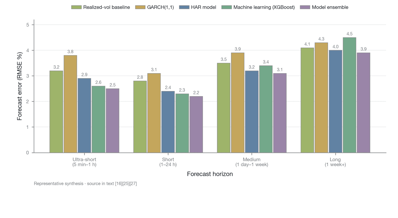
Figure 24-3. A comparison of forecast errors of volatility-forecasting models across time scales (representative composite illustration: the RMSE values shown are representative magnitudes synthesized from the literature, not exact values from any single source; data source: based on empirical studies of volatility forecasting in cryptocurrency and equity markets [16][25][27])
Each class of model has its own zone of comparative advantage: in the ultra-short-term window of 5 minutes to 1 hour, machine-learning models that process order book microstructure features directly (such as XGBoost) exhibit the lowest forecast error among the baseline models; in the short- to medium-term window of one day to one week, HAR models gradually surpass machine learning thanks to their multi-scale decomposition architecture; and once the forecast horizon exceeds one week, the errors of all classes of model converge, with mean reversion becoming dominant and complex models providing little incremental value. This pattern offers clear guidance for a model-combination strategy: emphasize machine learning in the short term, rely on HAR in the medium term, and respect mean reversion in the long term. Table 24-1 further summarizes, at the mechanistic level, the core features and applicable scenarios of each class of model in the perpetual futures market.
| Model class | Core mechanism | Perpetual-futures adaptation | Strengths | Weaknesses and limitations |
|---|---|---|---|---|
| Realized volatility | Sum of squared high-frequency returns | Bipower variation to remove jumps; handling of settlement pulses | Solid theoretical foundation; precise measurement | Only an ex post measure, not a direct forecasting model |
| GARCH | Autoregression of the conditional variance | Introduce a Student's t-distribution; combine with a jump-diffusion process | Captures volatility clustering; parameters are interpretable | Assumes a continuous process; struggles with liquidation jumps |
| HAR | Linear combination of multi-scale volatility | Add a funding-settlement cycle component and a liquidation-volume factor | Simple, robust structure; matches the stratification of market participants | Underfits extreme nonlinear interaction effects |
| Machine learning and deep learning | Nonlinear feature mapping and end-to-end learning | Fuse multidimensional heterogeneous signals (funding rate, order book, etc.) | Excels at ultra-short-term forecasting; captures complex nonlinear patterns | Black-box nature; very high risk of overfitting |
Table 24-1. Adaptation and evaluation of volatility-forecasting models in perpetual futures (data source: analysis of model characteristics [22][25][28])
Faced with the limitations of any single model, forecast combination offers a more robust solution. Taking a weighted average of the forecasts of several heterogeneous models can effectively diversify the risk that any individual model fails under a particular market state. The weights can be adjusted dynamically in inverse proportion to historical forecast errors, or set using an exponentially weighted moving average to give greater weight to models that have performed better recently. More important, quantitative models should be embedded within a three-layer risk-control framework that incorporates human judgment and hard stop-loss mechanisms, so that the system retains basic survivability when a model encounters a black swan event or a structural break [29].
24.3 A source-decomposed volatility forecasting framework
Forecasting the total volatility of the cryptocurrency market often runs into a structural dilemma: when we mix volatility from all sources together and try to fit it with a single unified model, volatility components of different natures interfere with one another, degrading forecast accuracy. The solution is not to seek an ever more complex unified model but to adopt a divide-and-conquer strategy. As Chapter 22 discussed, volatility in the perpetual futures market can be decomposed into four distinct sources: informational, liquidity, mechanical, and transmission volatility. Each source has entirely different drivers, time scales, and predictability characteristics. This section shows how to build a separate forecasting model for each of these four sources and then aggregate them into a forecast of total volatility; this framework constitutes the chapter's core methodological innovation.
The core idea of the source-decomposed framework derives from a basic principle of microstructure theory and signal processing: when multiple independent information sources drive an observed variable simultaneously, the optimal estimation strategy is to extract and process each source separately rather than to invert directly from the mixed signal. This principle is especially applicable in crypto markets, because the four volatility sources differ completely not only in physical mechanism but also in statistical properties. Informational volatility exhibits sparse, pulse-like behavior; liquidity volatility is strongly periodic; mechanical volatility is determined by protocol rules; and transmission volatility manifests as time-lagged cross-asset correlation. Attempting to capture all four properties with a single parameterized model amounts to asking one model to fit four data-generating processes with entirely different statistical characteristics, which inevitably lowers the efficiency of parameter estimation.
Figure 24-4 presents the complete architecture of the source-decomposed volatility forecasting framework in bottom-up logic: from the extraction of alternative signals at the base layer, to the independent modeling of the four volatility sources in the middle layer, to the variance aggregation and total-volatility forecast output at the top layer.
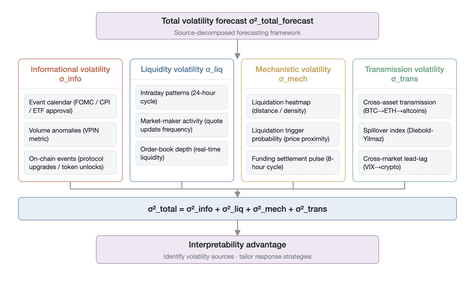
Figure 24-4. The conceptual architecture of the source-decomposed volatility forecasting framework (structural illustration, not measured data; data source: compiled by the author)
The core design principle of this architecture is embodied in three layers of information processing. At the base layer, different market signals (funding rate, liquidation heatmap, order book shape, on-chain data, and so on) are assigned to the volatility-source channel that best matches their physical mechanism, rather than being mixed as input to a single unified model. At the middle layer, each channel adopts the forecasting method best suited to its statistical properties: event-calendar regression for informational volatility, an HAR model for liquidity volatility, a threshold model for mechanical volatility, and a VAR spillover index for transmission volatility. At the top layer, the four independent forecasts are aggregated into a composite forecast of total volatility through variance summation and calibration of interaction terms. This layered processing ensures that the distinctive time scale and statistical properties of each volatility source are exploited to the fullest, rather than being averaged away in the parameter competition of a unified model.
24.3.1 Forecasting informational volatility
Informational volatility (σ_info) arises from the process by which new information reaches the market and is absorbed into prices. From a forecasting standpoint, informational volatility can be divided into a highly predictable component and an intrinsically unpredictable component. The predictable part consists mainly of the known event calendar, including macroeconomic data releases (such as Federal Open Market Committee (FOMC) decisions, Consumer Price Index (CPI) reports, and nonfarm payrolls data) and scheduled events specific to crypto markets (such as protocol upgrade dates, token unlock schedules, and exchange-traded fund (ETF) approval deadlines). Within the windows of these known events, the rate of information arrival to the market rises systematically.
Ben Omrane et al. (2025) [30] show that the volatility of Bitcoin and Ethereum reacts significantly and asymmetrically to macroeconomic data releases. Analyzing 5-minute-frequency data from 2016 to 2023, the study finds that volatility reacts significantly to only a few news categories, among which U.S. monetary policy news has a longer-lasting effect than the others. U.S. monetary policy news in particular drives volatility higher before, during, and after the announcement, and Ethereum is more sensitive to U.S. macroeconomic announcements than Bitcoin. This rise in volatility ahead of an announcement reflects participants adjusting their positions before the uncertainty is resolved, a phenomenon known as the pre-announcement volatility run-up effect. A forecasting model can therefore use event-calendar regression to automatically raise the baseline estimate of informational volatility during known event windows.
Concretely, one builds a piecewise event-calendar regression model. For each known macroeconomic event, a time window is defined—typically from 2 hours before to 4 hours after the release—and a dummy variable is set within this window. The model can be written as:
where D_{i,t} is the dummy variable for event i, and VPIN_t is the volume-synchronized probability of informed trading (VPIN), used to approximate the information arrival rate. The coefficients β_i and γ must be estimated empirically within-sample; their stability depends on the event type and market state, and they should not be applied directly across periods. VPIN was proposed by Easley, López de Prado, and O'Hara (2012) [31]; its essence is to divide trading volume into fixed-size volume buckets and estimate the degree of buy-sell order imbalance within each bucket to infer the active share of informed traders. Compared with the traditional probability of informed trading (PIN) model, it requires no maximum likelihood estimation and is more computationally efficient, and its volume-synchronized nature is naturally suited to the vast differences in activity across the 24/7 crypto market, avoiding the signal distortion of fixed time windows. This hybrid approach captures both the structured impact of known events and, through VPIN, changes in the information arrival rate outside event periods. One caveat is that in crypto markets VPIN is exposed to the contamination of volume by wash trading: at some exchanges wash trading may account for a substantial share, so a VPIN built on unfiltered volume develops a systematic bias. In practice, one should use wash-trading-filtered volume, or data from exchanges with a low share of wash trading, as input.
For informational volatility outside event periods, although there is no explicit calendar guidance, its baseline level is determined by the market's actual information arrival rate. In traditional microstructure theory, VPIN and volume anomalies are widely used to approximate the information arrival rate. When volume deviates markedly from its historical mean, or when buy and sell order flow becomes severely imbalanced, this usually signals an inflow of undisclosed information and thus foreshadows a near-term rise in informational volatility. The unpredictable component includes sudden "black swan" events such as regulatory raids, exchange bankruptcies, and protocol hacks. The timing of such events cannot be foreseen, so they cannot be incorporated into a point-forecast model and can only be addressed through a portfolio-level tail-risk budget.
In practice, on-chain events in crypto markets—such as protocol upgrades, major governance votes, and token unlocks—are also highly predictable. The dates of these events are typically announced weeks or months in advance, allowing participants to adjust their risk exposure ahead of time. Ethereum's major upgrades, such as the Shanghai and Dencun upgrades, for example, had their dates fixed months in advance, giving forecasting models a clear timing for the information shock.
24.3.2 Forecasting liquidity volatility
Liquidity volatility (σ_liq) is caused by changes in market depth and by market-maker behavior. Unlike informational volatility, liquidity volatility contains a large, highly predictable component. Most notable is the intraday pattern: the level of liquidity in crypto markets fluctuates with high regularity over a 24-hour cycle. Hansen et al. (2024) [32] find that crypto markets exhibit a clear intraday cycle in volatility and liquidity, a periodicity that is closely related to the activity of traders in different geographic time zones and to the execution times of algorithmic trading. For example, at the handover between the Asian and the European-American trading sessions, liquidity often reaches a trough, so that even a small order can trigger a large price move. The study further finds that crypto-market volatility and liquidity metrics exhibit pronounced intraday variation, which means that liquidity is highly predictable.
The mechanisms that produce this intraday liquidity pattern are several. First, traders in different time zones have clearly defined active hours: Asian traders are most active during Asian working hours, while European and American traders dominate during their working hours. During the handover between time zones (such as the gap between the Asian close and the European-American open), the number of participants falls to a trough, market makers' incentive to quote declines accordingly, and liquidity tightens noticeably. Second, the execution times of algorithmic trading are also highly regular: many institutional traders execute large orders at specific times (such as on the hour or half-hour), causing a sudden rise in liquidity demand at those points. Third, funding settlement times (though belonging to the category of mechanical volatility) also affect liquidity, because traders adjust their positions around settlement.
Beyond static time-of-day effects, market makers' real-time activity provides a dynamic forecasting signal. If the frequency with which market makers update their quotes suddenly drops, or the apparent depth of the order book begins to shrink, this usually signals that market makers perceive some latent risk and are reducing their risk exposure. Such defensive behavior is itself a strong leading signal that liquidity volatility is about to rise. In practice, one can track market makers' activity in real time by monitoring the quote refresh rate of the order book. Taking the BTC perpetual futures on a leading exchange as an example, when the quote refresh rate falls to 10% to 20% of its normal level, this usually presages an impending liquidity crunch.
In terms of forecasting method, the classic HAR model performs well in handling liquidity volatility. Brauneis and Sahiner (2026) [33] demonstrate that, although the HAR model effectively captures the clustering and long-memory features of volatility, forecast accuracy can be further improved by introducing machine-learning methods such as LightGBM (light gradient boosting machine) and XGBoost. The basic form of the HAR model is:
{t-6:t} + \beta_m \cdot \overline{RV}{t-29:t} + \varepsilon_t
where RV denotes realized volatility, and the subscripts denote the daily, weekly, and monthly scales, respectively. Here a crypto-market convention is used: the weekly term {t-6:t} is the average over the most recent seven calendar days and the monthly term {t-29:t} is the average over the most recent 30 calendar days—both including the current period t and thus consistent with the daily term —rather than the five and 21 trading days used in traditional finance. Even so, crypto-market participants still behave according to calendar cycles (weekend trading volume falls markedly, and intraday liquidity fluctuates regularly under the influence of geographic time zones), so the daily/weekly/monthly decomposition remains empirically effective; researchers need only note the difference in time-scale definitions when making cross-market comparisons. This multi-scale decomposition is naturally suited to forecasting liquidity volatility, because liquidity changes contain intraday, day-to-day, and week-to-week periodicity simultaneously. Within the source-decomposed framework, real-time order book depth, bid-ask spread skew, and market-maker activity can be fed as additional factors into an HAR or machine-learning model to fit the liquidity-volatility component specifically; when the state machine defined in Chapter 23 enters the "stressed" state, the model should automatically raise the baseline expectation for liquidity volatility.
24.3.3 Forecasting mechanical volatility
Mechanical volatility (σ_mech) is a feature unique to the perpetual futures market, created endogenously by protocol rules and the leverage-liquidation mechanism. Of the four volatility sources, mechanical volatility contains the most predictable deterministic component: the funding-settlement pulse. Funding settlement times are known: at traditional centralized exchanges such as Binance, settlement occurs every 8 hours (for example, at 00:00, 08:00, and 16:00 UTC), but a new generation of protocols has markedly increased the frequency—Hyperliquid and dYdX v4 both settle hourly, and Bybit has moved some contracts to settlement every 4 hours. Differences in settlement frequency directly shape the character of the mechanical-volatility pulse: a higher frequency means a smaller amplitude per pulse (because rate deviations are corrected over shorter intervals) but a greater frequency of pulses. Regardless of the specific frequency, the rate level is already observable in the order book and on derivatives data platforms before settlement. When the rate reaches an extreme level, arbitrageurs and directional traders concentrate their closing and opening of positions around settlement, either to avoid paying the high funding cost or to capture funding income. This foreseeable concentration of order flow inevitably produces a volatility pulse within the settlement window.
The settlement pulse can be forecast with a simple yet effective method. First, compute the deviation of the current rate from its historical mean; when the rate is at an extreme level (for example, an annualized rate above 100% or below −50%), the amplitude of the settlement pulse increases substantially. Second, monitor the speed of rate changes; the faster the rate moves, the stronger the market's directional bias and the greater the closing pressure at settlement. From the absolute level and rate of change of the current rate, the forecasting model can reasonably estimate the direction and magnitude of the settlement pulse. A simplified form of the model is:
where is the current rate, is its change, and is total open interest. The coefficients of this equation must be calibrated empirically within-sample and vary with the exchange's funding-settlement frequency and market state; they should serve as directional guidance rather than a ready-made fixed rule.
Another key source of mechanical volatility is the liquidation cascade. Although the triggering of a liquidation cascade is abrupt, its underlying risk distribution is highly transparent. By aggregating open-interest data across the entire market, a liquidation heatmap can precisely compute the scale of liquidations distributed at different price levels. The distance from the current market price to the nearest "liquidation cluster" is a powerful conditioning factor for forecasting mechanical volatility. For example, if the current Bitcoin price is $45,000, with $10 million of clustered long liquidations at $44,500 and $8 million of clustered short liquidations at $45,500, then these two price zones become high-risk areas.
A model for forecasting liquidation cascades should output a conditional volatility whose magnitude depends on the distance between the price and a liquidation cluster. A common approach uses a Gaussian kernel function to measure this distance:
where is the bandwidth of the Gaussian kernel, characterizing the price scale over which a liquidation cluster exerts influence; its dimension is the same as that of and (both a quote currency such as USD), not that of volatility. The larger the bandwidth, the more widely the cluster's influence spreads along the price axis. This form ensures that as the price approaches a liquidation cluster, the estimated mechanical volatility rises sharply. In real markets, liquidation clusters usually exist at several price levels simultaneously, and clustered long liquidations (concentrated below the current price) and clustered short liquidations (concentrated above it) are distributed asymmetrically. A more complete form of the model should therefore perform a kernel-density summation over all known liquidation clusters:
where is the center price of the k-th liquidation cluster, is the bandwidth corresponding to the k-th cluster (again a price scale), and the weight is determined by the estimated liquidation scale of that cluster. Note that, whereas the single-cluster equation treats as a multiplicative factor, the multi-cluster equation makes it an additive base: the kernel-summation term is added directly on top of the baseline volatility, so the two equations do not reduce to the same form even when only a single cluster is present. The liquidation-cluster data used here come from third-party estimates rather than precise exchange disclosures (as discussed in Section 24.1.3), so the model output is itself an estimate.
Forecasting liquidation cascades, however, has an inherent nonlinear boundary: whether a cascade will start can be predicted from the probability that the price approaches a liquidation cluster, but how violent the cascade will be once it starts is difficult to estimate precisely. This is because the intensity of a cascade depends on the order book liquidity at the moment of triggering, and that liquidity evaporates rapidly once the cascade begins. This "liquidity evaporation" was especially evident in the March 2020 crypto crash, when Bitcoin fell by more than 50% within a few hours and triggered a liquidation cascade of several billion dollars. A model for mechanical volatility should therefore output an asymmetric probability distribution: as the price approaches a liquidation cluster, the model must not only raise the mean forecast of volatility but also substantially increase the probability weight on extreme tail movements. This is usually achieved by using a Student's t-distribution or a generalized Pareto distribution.
24.3.4 Forecasting transmission volatility
Transmission volatility (σ_trans) reflects the spread of a shock from one asset or market to another. This transmission is not instantaneous but involves a physical delay of minutes to hours, and that delay provides an exploitable time window for volatility forecasting. At the macro level, volatility in traditional financial markets often leads that in crypto markets. For example, when the VIX—the implied volatility of S&P 500 options—rises sharply or U.S. Treasury yields jump, crypto-market volatility typically responds within minutes to hours, and this transmission lag has been shrinking steadily as institutional capital enters crypto through the ETF channel. Moreover, the direction of transmission is not always one-way: in certain events, such as the 2022 FTX collapse, crypto-market volatility can also propagate back to traditional financial assets. This increasingly tight and bidirectional cross-market linkage means that forecasting transmission volatility must incorporate the two-way spillover paths between traditional finance and crypto markets.
Within crypto markets, clear lead-lag relationships also exist among assets. As the market's liquidity anchor and the representative "risk asset," Bitcoin's volatility increases often lead Ethereum's and then propagate to less liquid altcoins. This transmission lag is typically minutes to hours, depending on each asset's liquidity depth and the attention traders pay to it. Shahrour et al. (2025) [34] quantify this cross-market spillover using a time-varying parameter vector autoregression (TVP-VAR) technique and find that, within their particular sample period and asset set, Bitcoin and the NEAR protocol are the main transmitters of volatility, influencing 68.17% and 71.63% of other assets' volatility, respectively, whereas traditional financial instruments such as Treasury bills act more as net receivers of volatility. The finding that NEAR's spillover influence exceeds Bitcoin's may reflect the particular asset selection and sample-period bias of that study; because NEAR's market capitalization and liquidity are far smaller than BTC's, whether such a high spillover coefficient is robust across different samples remains to be tested.
To exploit this transmission mechanism systematically within a forecasting model, one can introduce a real-time version of the Diebold-Yilmaz spillover index. Through variance decomposition, this index dynamically measures "who is transmitting volatility to whom" and the strength of that transmission. The Diebold-Yilmaz index is computed from the variance decomposition of a vector autoregression (VAR, to be distinguished from value at risk, VaR) model:
where is the contribution of a shock to asset to the variance of asset , and is the Diebold-Yilmaz spillover index. When the monitoring system detects a sharp rise in the overall spillover index, or a marked strengthening of the directional spillover from a particular asset (such as Bitcoin) to others, the forecasting model should automatically raise the estimated transmission volatility of the target asset. This approach converts changes in the cross-market topological structure into direct inputs for volatility forecasting.
24.3.5 Aggregating the four-source forecast
Once the four volatility sources have been forecast independently, the forecast of total volatility can be obtained by summing the variances of the individual forecasts (plus empirically calibrated interaction terms). This source-decomposed aggregation is significantly superior, both in theory and in practice, to a unified model that forecasts total volatility directly. The aggregation formula is:
{\text{info}} \cdot \hat{\sigma}{\text{liq}} + \cdots
where is an empirically calibrated interaction coefficient. In practice, these interaction terms are usually small, because the drivers of the four volatility sources are relatively independent.
The reasonableness of the four-source independence assumption depends on the state the market is in. In a calm state, the drivers of the four volatility sources do indeed differ fundamentally: informational volatility is driven by the news arrival rate, liquidity volatility by market-maker behavior and the intraday cycle, mechanical volatility by funding settlement and liquidation trigger conditions, and transmission volatility by cross-market fund flows. Under normal market conditions, these drivers are weakly correlated, so the interaction terms contribute little to the total forecast.
In a crisis state, however, the independence assumption may be significantly violated. When a major information shock (such as a sudden regulatory action) simultaneously triggers a sharp price drop, the withdrawal of liquidity providers (liquidity volatility), the triggering of liquidation clusters (mechanical volatility), and cross-asset panic transmission (transmission volatility) may all activate synchronously within minutes. In such an extreme scenario, the interaction terms among the four volatility sources may account for a significant share of total variance, and simple variance summation will underestimate the true total volatility. Both the "Black Thursday" of March 2020 and the 2022 FTX collapse exhibited this feature of synchronous multi-source activation. Feasible ways to handle this limitation include introducing state-dependent interaction coefficients that automatically amplify the interaction-term weights when the state machine identifies a "stressed" or "crisis" state, or adopting a conditional-correlation structure (such as a dynamic conditional correlation (DCC) model) to model the time-varying correlations among the four volatility sources. This limitation is a known structural constraint of the framework, and readers should pay particular attention to the reliability of the model's output in a crisis state.
Moreover, the decomposition into four volatility sources is not, in the statistical sense, a unique decomposition. Different decomposition methods (such as principal component analysis, independent component analysis, or attribution based on different microstructure feature sets) may yield different definitions of the "four sources" and different independence properties. This framework's decomposition rests on the physical-mechanism prior classification proposed in Chapter 22—information arrival, liquidity supply, protocol rules, and cross-market transmission—which gives it a relatively stable economic meaning across different samples and model specifications rather than being a purely statistical artifact. In day-to-day operation, however, precise attribution still faces the challenge of multicollinearity: a single large liquidation (mechanical) may simultaneously alter order book depth (liquidity) and transmit through cross-asset positions to other markets (transmission), so the boundaries of attribution are inevitably blurred. In practice, source-decomposed forecasts should be treated as an approximate tool that provides directional guidance rather than a quantitative decomposition accurate to the decimal point.
Table 24-2 systematically compares the differentiated positioning of the four volatility sources within the forecasting framework along three dimensions—predictability profile, core predictors, and optimal forecasting method: the four have almost no overlap in the source of their predictability, their time scale, or their optimal mathematical tool.
| Volatility source | Predictability profile | Core predictors | Optimal forecasting method |
|---|---|---|---|
| Informational volatility (σ_info) | High during event windows, low otherwise | Macro event calendar, VPIN, on-chain events | Event-calendar regression + order-flow imbalance model |
| Liquidity volatility (σ_liq) | Strongly periodic, highly predictable | Order book depth, market-maker quote frequency, time of day | HAR model with depth features / machine learning |
| Mechanical volatility (σ_mech) | Conditionally triggered, highly nonlinear | Funding rate level, distance on the liquidation heatmap | Threshold model + extreme value theory (EVT) |
| Transmission volatility (σ_trans) | Time-lagged, traceable | VIX index, cross-asset lead-lag relationships | Diebold-Yilmaz spillover index + VAR |
Table 24-2. A comparison of the forecasting characteristics and methods of the four volatility sources (data source: compiled by the author)
The reason divide-and-conquer outperforms a unified model is, fundamentally, that it avoids feature confusion during model learning. A unified GARCH or machine-learning model tries to make the same set of parameters learn the 8-hour funding pulse, the 24-hour intraday liquidity pattern, and the multi-day macro transmission all at once. Such multi-scale, multi-driver mixed input often leaves the model wavering between states, ultimately producing a mediocre mean forecast. Source-decomposed forecasting, by contrast, allows the most suitable mathematical tool and time scale to be chosen for each physical mechanism.
Another core advantage of source-decomposed forecasting is its interpretability. When a unified model forecasts that tomorrow's volatility will reach 80%, a market maker knows only that risk has increased, not how to respond. A source-decomposed model, by contrast, can state explicitly whether the rise in volatility is because "the price is only 2% away from a large-scale liquidation cluster" (mechanical volatility dominant), because "there is an FOMC rate decision tomorrow evening" (informational volatility dominant), or because "the VIX index has spiked suddenly and cross-market spillover has strengthened" (transmission volatility dominant). Different attributions lead directly to different trading and risk-control decisions: if liquidation risk dominates, a trader may choose to reduce leverage or adjust the direction of the position; if a macro event dominates, the trader may choose to increase position size but lower leverage; if cross-market transmission dominates, the trader may choose to hedge the exposure to the source asset. This is precisely the core value of turning volatility theory into an engineering application.
Figure 24-5 makes the case for the source-decomposed framework along two dimensions: the left panel compares the forecast errors of the source-decomposed aggregation method against a traditional unified GARCH model across four time windows, while the right panel reports the predictability of each of the four volatility sources—together giving intuitive support for the decomposition strategy.
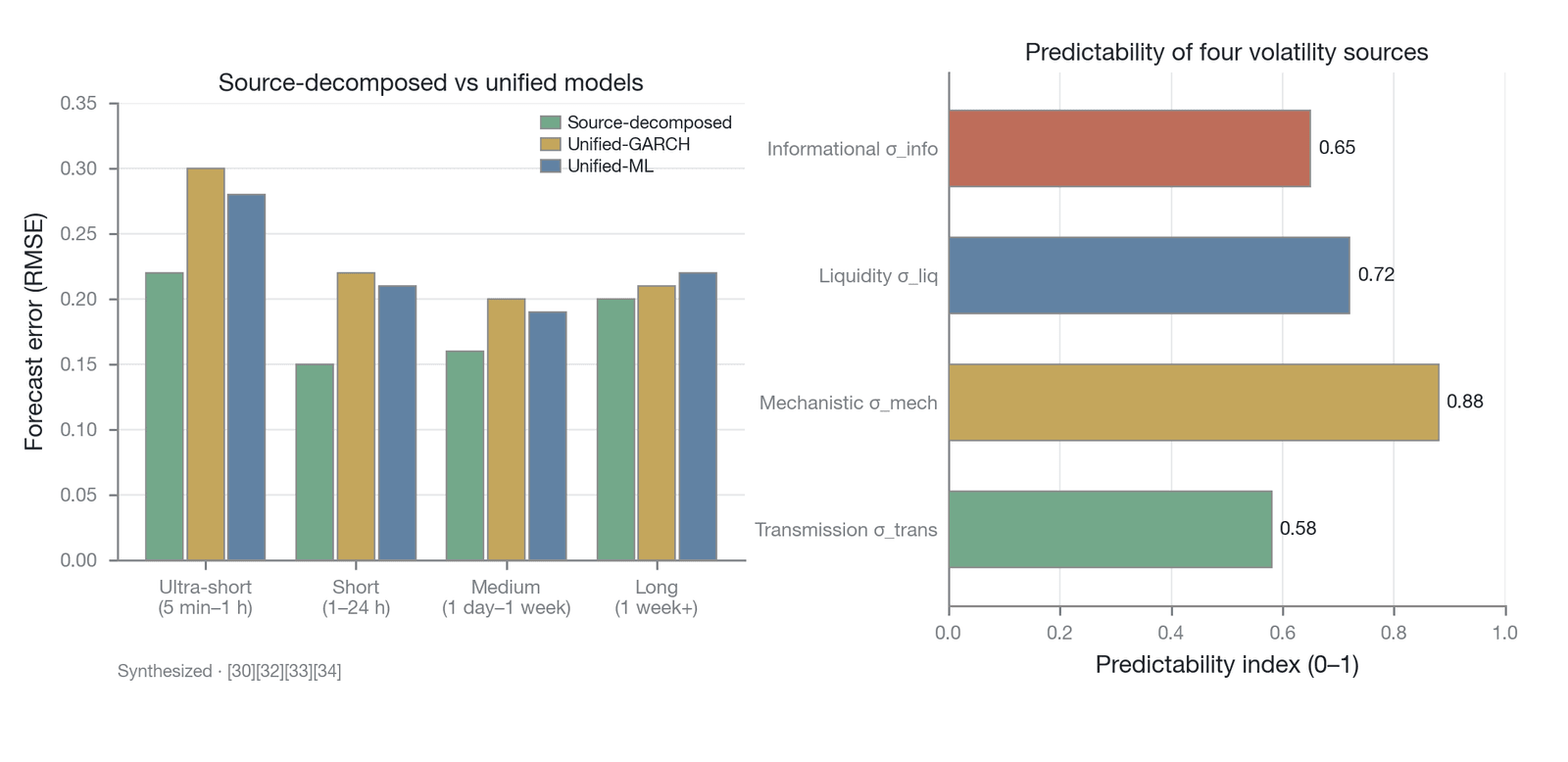
Figure 24-5. A performance comparison of source-decomposed and unified-model forecasting, and the predictability of each source (illustrative synthesis extrapolated from the literature, not independent empirical evidence: the RMSE and predictability values shown are relative magnitudes, not measured data; data source: the author's synthesis based on the literature [30][32][33][34])
Building on the above literature's empirical findings on crypto-market volatility forecasting, this book extrapolates the performance advantage of the source-decomposed aggregation method over a unified model. In ultra-short-term (5 minutes to 1 hour) and short-term (1 to 24 hours) forecasting, the source-decomposed method is expected to achieve a significant improvement in error, because at these time scales the periodic features of liquidity volatility and mechanical volatility are especially pronounced and the source-decomposed method can capture these regularities precisely. In medium- and long-term forecasting, the advantage is expected to weaken but to still preserve some improvement in error. These performance estimates are conceptual judgments synthesized from the literature, not independent empirical conclusions.
Moreover, based on the physical mechanisms of each volatility source and the qualitative analysis in the literature, the predictability of the four volatility sources differs systematically, ranging from highest to lowest as follows: mechanical (funding settlement times are fixed and the liquidation heatmap is transparent), liquidity (the intraday pattern is highly regular; Hansen et al. (2024) [32] document a pronounced intraday periodicity), informational (the event calendar is known, but information arrival outside events remains random), and transmission (the lag and strength of cross-market transmission vary considerably). This systematic difference in predictability across sources further supports source-decomposed modeling over unified modeling.
The performance advantage of the source-decomposed forecasting framework described above currently rests on theoretical extrapolation and a synthesis of the literature and awaits independent empirical testing. An ideal validation scheme should contain the following elements: at the sample-asset level, coverage of perpetual futures data for at least BTC, ETH, and two or more altcoins; in terms of time span, coverage of a complete bull-bear cycle (at least three years is recommended) including at least two known liquidation-cascade events; at the benchmark-model level, a standard GARCH(1,1), an HAR-RV, and a unified machine-learning model as control groups; and in terms of evaluation metrics, simultaneous reporting of root mean square error (RMSE), mean absolute error (MAE), and a quantile loss function, evaluated separately across different time scales (intraday, daily, weekly). This validation work constitutes the key follow-up research direction for taking the framework from theory to empirical evidence.
The four outputs of the source-decomposed forecasting framework—the independent estimates of informational, liquidity, mechanical, and transmission volatility—constitute the core inputs to the subsequent three-layer decision system. At the micro level, market makers dynamically adjust their quoting strategy based on real-time identification of the volatility source; at the meso level, directional traders and portfolio managers use source-decomposed forecasts for position sizing and tail-risk management; at the macro level, exchanges and protocol designers embed the forecast signals in dynamic margin calibration and liquidity early-warning systems. The following three sections develop the specific applications of these three levels in turn.
24.4 Applying volatility in market-making decisions
Market makers are the most direct consumers of volatility forecasts, and every gain in forecast quality translates into a better quoting decision. This section connects the market-making profit equation of Chapter 19 with the volatility analysis of Chapters 22 through 24 to show how such knowledge enters real-time decision-making.
24.4.1 Volatility and the optimal spread
Starting from the profit equation of Section 19.1.4, the market maker's profit structure comprises four core parts: market-making profit equals spread revenue minus adverse-selection loss, minus inventory-volatility loss, and finally minus institutional cost. This equation provides a basic framework for understanding how volatility affects market-making decisions. The different components of volatility have asymmetric effects on the terms of the profit equation. Adverse-selection loss is positively related to informational volatility: when informational volatility rises, informed traders are more active in the market and the adverse-selection risk faced by market makers rises accordingly. Inventory-volatility loss is positively related to total volatility, and the relationship between the two is markedly convex [35]. When total volatility doubles, the risk cost of a market maker holding inventory rises by more than a factor of two. In addition, institutional cost is positively related mainly to mechanical volatility: extreme events such as liquidation cascades significantly increase a market maker's potential loss in the tail.
The setting of the optimal spread must dynamically reflect this nonlinear risk structure. Theoretical models show that a market maker's optimal spread should widen nonlinearly as volatility rises. Wyart et al. (2008) established, in order-driven markets, that the bid-ask spread is approximately proportional to volatility [35], and under an inventory-risk-based optimal market-making framework the optimal spread contains a nonlinear term directly related to the variance of volatility [36]. This book adopts an illustrative elasticity range slightly above 1 (roughly 1.2 to 1.5) to characterize the convex sensitivity of the spread to volatility; this range is an illustrative modeling assumption rather than a figure from any single empirical source, and given the higher leverage and more extreme liquidity swings of perpetual futures, the actual elasticity coefficient may deviate from this range and awaits independent validation in the crypto perpetual futures market. This implies that when realized volatility rises by 10%, a market maker seeking to remain risk-neutral should widen the optimal quoted spread by 12% to 15%. Figure 24-6 shows the convex relationship between volatility and the optimal market-making spread derived from this theory.
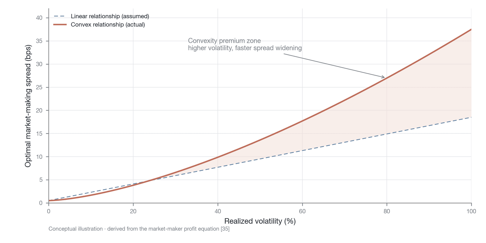
Figure 24-6. The convex relationship between volatility and the optimal market-making spread (theoretical-derivation illustration, not measured data: the elasticity of roughly 1.2 to 1.5 is an illustrative modeling assumption and awaits independent validation for crypto perpetual futures; data source: derived theoretically from the market-maker profit equation [35])
The convex curve in Figure 24-6 carries a concrete practical implication: spread adjustment cannot follow a simple linear mapping but must build in acceleration, so that once the volatility forecast breaks through a threshold, the pace at which the spread widens itself accelerates. A market-making system that handles this convexity poorly will suffer severe adverse-selection losses in the critical interval where volatility jumps from moderate to extreme.
24.4.2 State identification and strategy switching
The state-machine model proposed in Chapter 23 has direct engineering value in market-making strategy. Rather than using one set of static parameters to cope with all market environments, a market maker switches dynamically among three distinct market-making modes based on the volatility state. In the calm state, where volatility is at a historical low with no clear upward trend, the market-making system runs in standard mode, characterized by extremely narrow spreads, deep order book depth, and an active willingness to fill orders, with the goal of maximizing spread revenue. When volatility breaks through the first threshold and enters the stressed state, the system automatically switches to defensive mode. Here the spread typically widens by 50% to 100%, the resting depth at each price level is halved, and inventory limits are tightened sharply. If volatility continues to surge and triggers the crisis state, the market-making system enters minimal-market-making or market-making-suspension mode, quoting extremely wide spreads or withdrawing orders entirely, placing the protection of capital first.
Figure 24-7 integrates the switching logic, trigger conditions, and effects on quoted spread, order book depth, and inventory limits of these three market-making modes into a single decision flowchart. State identification in real time draws on signals across several dimensions: the system tracks not only the level and trend of current realized volatility but also the leading signals discussed in Section 24.1—the proximity of the liquidation heatmap and micro-level changes in order book shape—which together let the state machine estimate the most probable current market state on the fly.
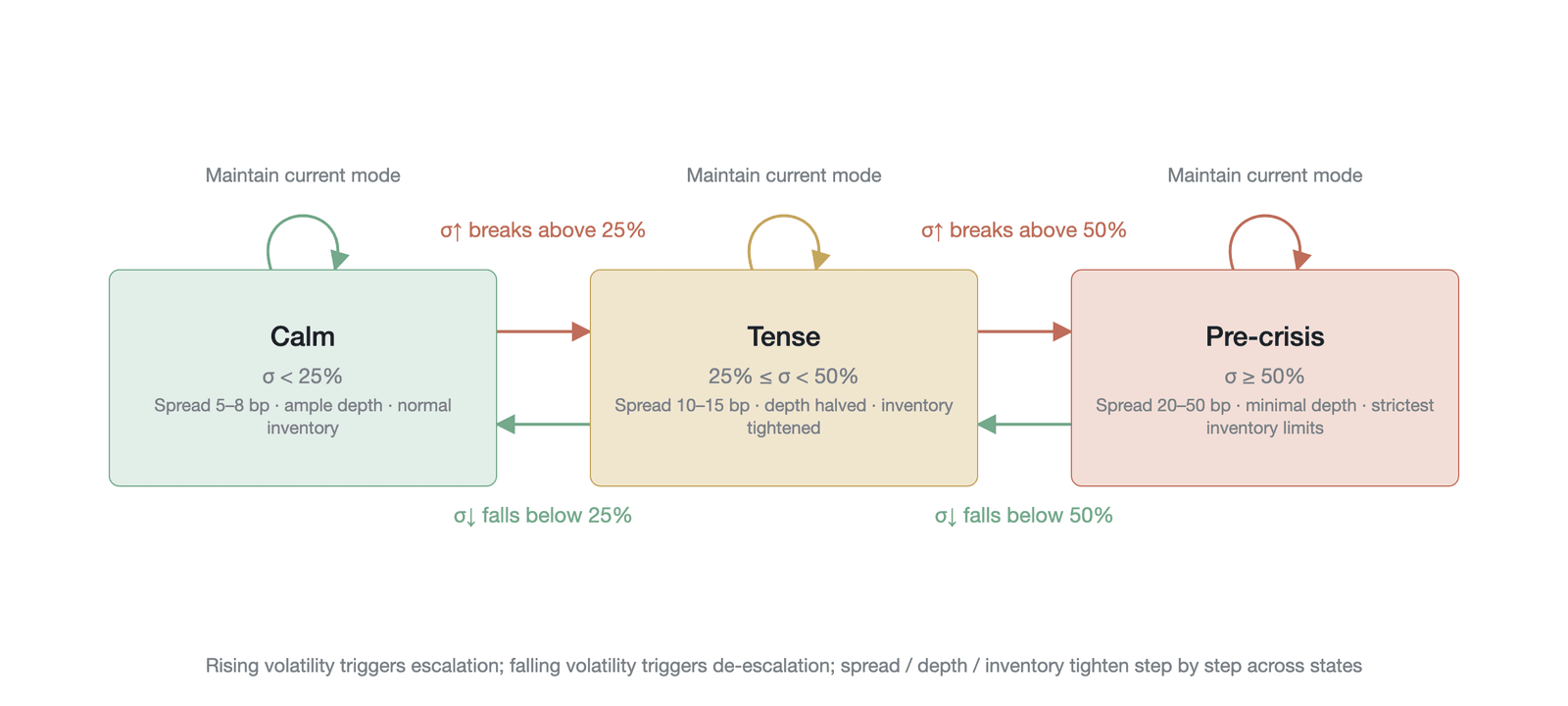
Figure 24-7. Volatility-triggered switching of a three-mode market-making strategy (structural illustration, not measured data: the three bands σ < 25%, 25% to 50%, and σ ≥ 50% are illustrative regime thresholds introduced by this figure and are not stated in the main text; data source: extrapolated from an application of the state-machine model [37])
The figure makes clear that switching among the three modes is not a symmetric design. The threshold for switching from calm to stressed is deliberately set at a relatively low volatility level, making the system highly sensitive to rising risk; the threshold for returning from stressed to calm is set markedly lower, forming a hysteresis window. The core reason for this asymmetry is that a market maker would rather bear the potential profit loss of defending too early than be exposed to enormous adverse-selection risk when volatility erupts; the system must confirm that volatility has substantively fallen back and that liquidation risk has completely receded before it gradually relaxes inventory limits and narrows spreads, so as to prevent a second loss from resuming normal market-making too early during a volatility aftershock.
24.4.3 Distinguishing liquidation volatility from informational volatility
When facing a sharp price drop, a market maker confronts the core difficulty described in Section 19.4.3: it must judge, within an extremely short interval, whether the current plunge is driven by informed trading or triggered by a liquidation cascade. The optimal responses to these two cases are exactly opposite. If the drop is driven by informed trading, this means the asset's fundamentals have changed, the price will not revert in the short term, and a market maker that fills orders will face a certain adverse-selection loss, so the optimal strategy is to withdraw immediately. If the drop is driven by a liquidation cascade—a form of mechanical volatility—the price often rebounds once the liquidation selling pressure is exhausted, so although filling orders entails short-term inventory risk, the expected return is very high.
Decomposing the volatility signal provides a key tool for distinguishing these two scenarios. An informed-trading-driven drop is usually accompanied by a rise in the volume-synchronized probability of informed trading, an increase in permanent price impact, and a refusal of the price to mean-revert after the shock, which manifests as a marked rise in the informational-volatility component. A liquidation-driven drop, by contrast, manifests as a spike in liquidation volume, a sharp fall in open interest, and an amplification of transitory price impact, corresponding to a surge in the mechanical-volatility component [38]. Figure 24-8 uses a decision tree to show how a market-making system, based on real-time signals across multiple dimensions—including the rate of change of liquidation volume, the change in open interest, the VPIN value, and the persistence of price impact—makes a millisecond-level choice between two entirely different response strategies.
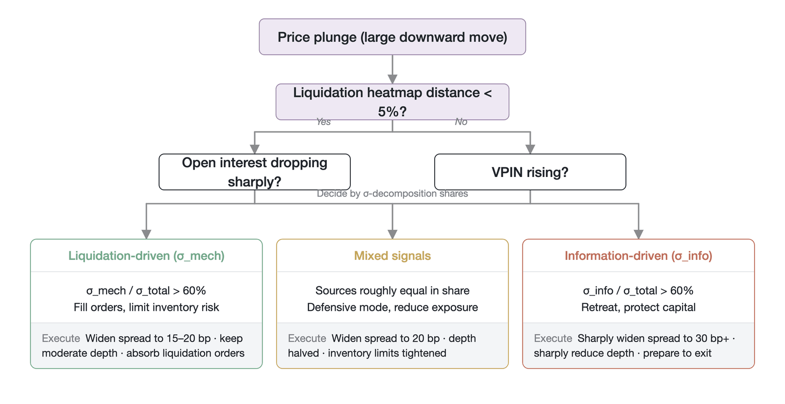
Figure 24-8. Real-time signals for distinguishing liquidation volatility from informational volatility (structural illustration, not measured data: the ratio of mechanical volatility to total volatility uses 60% as a simplified illustrative threshold; data source: extrapolated from the volatility-decomposition framework [38])
The core branching logic of the decision tree is that liquidation-driven and information-driven drops are highly distinguishable at the microstructure level: a liquidation event is accompanied by a sharp contraction of open interest, whereas in an information event open interest usually remains stable or even increases. The market-making system accordingly computes the ratio of mechanical volatility to total volatility in real time; if this ratio exceeds a preset threshold (60% as a simplified example), it judges the move to be driven mainly by liquidations and leans toward staying in the market and absorbing liquidation orders. Conversely, if the share of informational volatility exceeds the threshold, it judges the move to be an information-driven structural decline and triggers the withdrawal mechanism. In practice, real systems use a probabilistic soft threshold—a Bayesian posterior probability, say—rather than a hard cutoff, because the four-source decomposition must run in real time, entails a computational delay of hundreds of milliseconds to seconds, and loses considerable accuracy in extreme conditions.
24.4.4 Risk management for protocol market-making vaults
Automated market-making mechanisms at the protocol level face challenges different from those of traditional market makers. Take Hyperliquid's Hyperliquidity Provider (HLP) vault as an example: as the protocol's native liquidity provider, it bears responsibility for supplying baseline liquidity to the entire platform. Unlike traditional high-frequency market makers, which can exit the market at any time, HLP is designed to provide liquidity continuously in normal operation [39]. Although liquidity providers (LPs) can submit redemption requests (subject to a lock-up period and a queue), and although in extreme circumstances governance mechanisms such as validator voting can intervene to adjust operating parameters (the JELLY incident of March 2025 being one such intervention), HLP is designed to keep running under the vast majority of market conditions. Being unable to withdraw, however, does not mean abandoning risk management; HLP achieves a volatility-driven degradation mode by dynamically adjusting its strategy parameters.
When the risk indicators output by the volatility-forecasting model exceed a warning threshold, the HLP vault automatically triggers a degradation mechanism. This mechanism comprises three levels of response: first, the quoted spread automatically widens several-fold according to the volatility level, to compensate for the sharply rising adverse-selection risk; second, the resting depth on each side of the order book shrinks to a small fraction of its normal level, strictly limiting the maximum inventory that could accumulate in a one-sided market; and finally, the system suspends market-making on high-volatility altcoins, concentrating its limited capital on the most liquid, most controllable core assets [40]. This do-not-withdraw-but-degrade philosophy is precisely the concrete implementation of the crisis behavior of market-making vaults discussed in Section 21.4.2. The volatility-forecasting model constitutes the core engine driving this degradation mechanism, ensuring that the protocol dynamically balances the provision of baseline liquidity against the protection of liquidity providers' capital. A decentralized market-making vault also faces a risk dimension that centralized exchange (CEX) market makers do not: oracle dependence. HLP's mark-price computation and liquidation triggering rely on oracle inputs, and if the oracle is manipulated or delayed, the vault's entire risk-control logic can be bypassed. In the 2023 Mango Markets incident, an attacker manipulated the oracle price and caused protocol-level losses exceeding $100 million, showing that the trust-stack risk faced by decentralized exchange (DEX) market-making vaults (from oracle to mark price to liquidation triggering) differs structurally in nature from the risk faced by CEX market makers.
24.5 Applying volatility in directional trading and portfolio management
Volatility is not only a core input for market makers setting spreads and managing inventory; directional traders and portfolio managers likewise rely on volatility information to decide on position size, risk exposure, and stop-loss settings. In the perpetual futures ecosystem, which lacks a deep options market, participants cannot isolate and trade volatility risk directly through options. This missing market structure requires traders and portfolio managers to use indirect means to achieve volatility adjustment, volatility timing, and tail-risk management. The core argument of this section is that the application of volatility information is not an optional optimization but a basic competency that perpetual futures participants must master. For individual traders and institutional portfolio managers alike, the degree to which they understand volatility directly determines their probability of survival in a high-risk market.
24.5.1 Volatility-adjusted position sizing
The Kelly formula is a classic method in quantitative trading for determining the optimal position size; its core logic is that the optimal position size is proportional to the strategy's reward-to-risk ratio [41]. In the standard discrete form, the Kelly formula is , where is the strategy's win probability, is the loss probability ($1 - p$), and is the average win-loss ratio. In the continuous case, when returns follow a normal distribution, the Kelly criterion generalizes to , where is the expected excess return and is the return variance. The logic of the generalization from discrete to continuous is that as trading frequency tends to infinity and the return per trade tends to zero, the limiting form of the discrete Kelly formula converges to the continuous expression , which also intuitively shows that the optimal position is proportional to expected return and inversely proportional to the square of volatility (on the effect of betting frequency on the long-run performance of a Kelly strategy, see [42]). The deeper implication is that, by maximizing the expected growth rate of log wealth, the formula identifies the position size that minimizes the probability of ruin in long-run trading [41]. In the crypto perpetual futures market, however, the return distribution exhibits pronounced fat tails (with kurtosis far above that of the normal distribution), and applying the classical Kelly formula directly often leads to excessive position sizes. In practice, one usually applies a conservative correction via fractional Kelly—investing only 50% to 75% of the Kelly-optimal fraction—in exchange for a markedly lower probability of ruin and a smoother equity curve. The theoretical rationale for fractional Kelly is that when the return distribution departs from the normal assumption (especially in the presence of fat tails), the actual risk of full Kelly is far higher than the model predicts, and moderately reducing the fraction can greatly improve worst-case performance at the cost of only a small sacrifice in long-run growth rate [43].
Volatility adjustment in perpetual futures requires the four-source-weighted forecast rather than simple historical volatility. As Chapter 22 discussed, the four volatility sources carry entirely different implications for trading decisions. Informational volatility may accompany a directional trading opportunity, because the price is moving toward a new fundamental equilibrium; mechanical volatility (such as a liquidation cascade) and liquidity volatility, by contrast, are usually pure microstructure noise. If the forecast shows that the future rise in volatility is driven mainly by mechanical volatility, the trader should sharply reduce position size to avoid being liquidated by disorderly price jumps; but if the rise is caused by an information shock and the trader's strategy itself depends on capturing fundamental trends, the reduction in position size should be relatively small. The two differ significantly in the direction and magnitude of their effect on position size. This source-decomposed approach to position adjustment is more refined than mechanically reducing positions according to the level of total volatility, and it better fits the actual risk profile of the trading strategy.
The compounding effect of leverage further complicates position-sizing decisions in perpetual futures. In traditional equity markets, reducing position size usually means reducing the notional principal; in the perpetual futures market, however, a trader faces a choice along two dimensions—reducing notional principal and reducing the leverage ratio. In a high-volatility environment, reducing the leverage ratio is more critical than merely shrinking the notional principal. This is because high leverage significantly shortens the liquidation distance, and nonlinear jumps in volatility can easily trigger the liquidation mechanism. As a concrete example, suppose a trader holds a $10 million notional BTC long at 10x leverage, with a liquidation distance of about 10% of the current price. If volatility jumps from a normal 30% to 100% (which is common in a liquidation cascade), the price could fall by more than 12% within a few hours—enough to trigger liquidation. Even 10x, a relatively conservative level of leverage, still carries substantial forced-liquidation risk in an extreme volatility environment, and the risk at higher leverage is naturally more severe. Rules of thumb from practice indicate that there is a convex relationship between volatility and extreme loss: when volatility doubles, in order to maintain the same probability of ruin, position size should be reduced not merely linearly to 50% of the original but usually to between 50% and 70% of it [43]. This range is an empirical estimate from trading practice; the exact value depends on the fat-tailedness of the return distribution and the leverage actually used, and should not be applied as a hard rule. This convexity comes from the nonlinear nature of risk: the loss under extreme volatility is not merely a linear multiple of the loss under normal volatility.
Figure 24-9 shows the nonlinear relationship between the level of volatility and the Kelly-optimal position fraction. This convexly decreasing curve is one of the most important reference benchmarks for perpetual futures traders in managing position size.
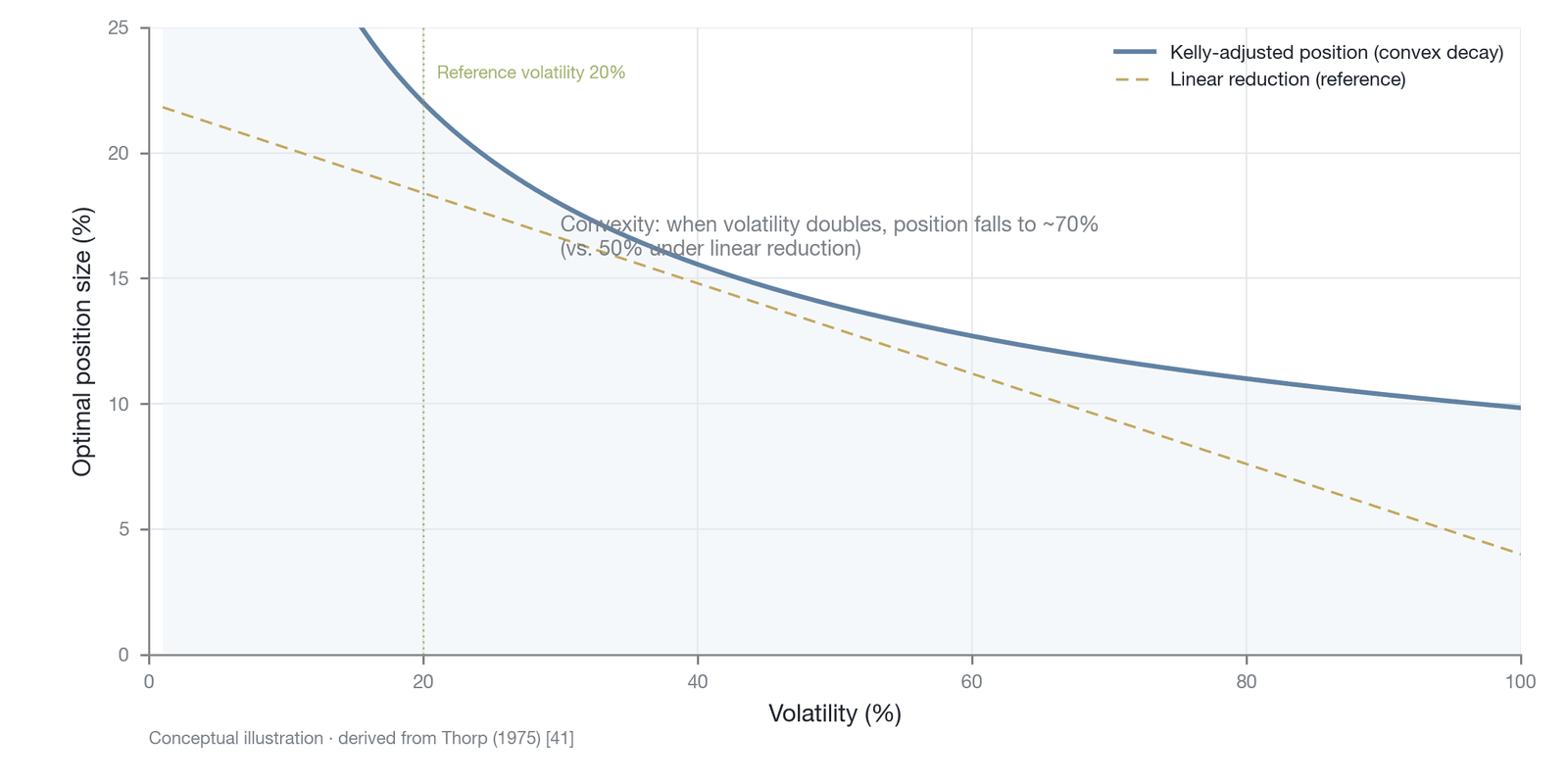
Figure 24-9. The convex function of Kelly position size adjusted for volatility (theoretical-derivation illustration, not measured data: the curve is an illustrative convex decline in which a doubling of volatility reduces position size to roughly 70%, aligned with the fractional-Kelly rule of thumb of 50% to 70% in the main text [43]; the Kelly criterion follows the theoretical derivation of Thorp 1975 [41])
The convexity in the figure has direct practical implications. In the low-volatility interval (such as 20% to 40% annualized), the curve's downward slope is steepest and position size is most sensitive to changes in volatility; when volatility enters the high interval (such as above 80% annualized), the slope flattens markedly, and although position size continues to fall, the marginal reduction per unit change in volatility shrinks. In the extreme volatility environment peculiar to crypto markets (where annualized volatility can exceed 200% during a liquidation cascade), this curve approaches zero, conveying a clear message: from the standpoint of long-run capital growth, maintaining any significant directional position amid extreme volatility is irrational.
24.5.2 Volatility timing
Volatility-timing strategies rest on the premise that market volatility exhibits identifiable regime shifts. As in the state-machine model constructed in Chapter 23, the market switches among three states—calm, stressed, and crisis. Directional traders can dynamically adjust their risk exposure by identifying these state transitions, thereby reducing drawdowns while improving risk-adjusted returns [37]. The key advantage of the state-machine model is that it does not try to predict the absolute level of volatility but instead identifies qualitative changes in market structure. Such identification is often more reliable than a precise volatility forecast, because transitions in market structure usually produce observable signals.
When the market moves from the calm state into the stressed state, the optimal response is to reduce directional risk exposure and raise the cash allocation. The stressed state is usually accompanied by thinning order book depth and extreme funding rates, which not only increases the slippage cost of trading but also raises the probability of mechanical volatility. At this stage, many traders' intuitive reaction is to double down, hoping to capture larger gains amid high volatility. This approach, however, often leads to severe losses, because the stressed state itself signals the fragility of market structure, in which any small shock can trigger a chain reaction. If the market deteriorates further in the stressed state and approaches the crisis state, the trader should reduce risk further or establish explicit hedging positions. The crisis state is characterized by a sharp rise in cross-asset correlation, and traditional diversification often fails at such times because all assets fall in unison. In this situation, holding positions in multiple different crypto assets provides no effective diversification protection.
The transition period from the crisis state back toward the stressed state is often the best window for contrarian traders and mean-reversion strategies to step in. In extreme events such as liquidation cascades, volatility usually overreacts and the price is pushed away from its fundamental equilibrium. As liquidity begins to recover and market risk aversion recedes, this mean-reversion tendency of volatility offers liquidity providers and reversal traders trading opportunities with highly asymmetric returns [44]. In the "Black Thursday" of March 2020 and the June 2022 Luna collapse, traders who established long positions at what proved, with hindsight, to be the optimal entry point earned short-term returns exceeding 200% over the subsequent days to weeks (BTC, for instance, rebounded from a low of about $3,800 on March 12, 2020, and some altcoins staged oversold rebounds after the June 2022 Luna collapse). This figure, however, suffers from severe survivorship bias: in live trading, participants cannot know whether the current price is the bottom. In the March 2020 event, many traders who tried to buy the dip at the $5,000 to $6,000 level were liquidated by the subsequent decline, and only the few who had reserved an ample margin buffer ultimately profited. In practice, volatility-timing strategies face a core pitfall: state transitions in volatility are not knowable instantaneously and can only ever be confirmed statistically after the fact. In live trading, state identification entails an unavoidable delay, and a strategy's design must be able to tolerate the friction cost of this delay; otherwise, frequent misjudgments and repeated repositioning will erode all of the strategy's excess return.
24.5.3 Indirect volatility trading in perpetual futures
In traditional financial markets, the core instrument for volatility trading is the option; traders can build pure volatility exposure by buying or selling a straddle or by trading volatility-index futures (such as VIX futures) directly [45]. An option's sensitivity to volatility—its vega exposure—enables traders to isolate volatility risk precisely, independent of the underlying asset's directional movement. In the crypto options market, which lacks depth, perpetual futures traders must construct strategies that are long or short volatility through indirect means. The core logic of these indirect strategies is to exploit the microstructure features peculiar to perpetual futures to capture changes in volatility.
The calendar-spread volatility strategy is a method of trading volatility indirectly by using funding-rate forecasts. When future market volatility is expected to rise sharply, the volatility of the funding rate usually rises with it. A trader can build long-short funding-rate positions across different perpetual futures (such as the same asset on different exchanges, or highly correlated assets within the same ecosystem). The return on this strategy does not depend on the absolute price direction of the underlying asset but on the realized volatility of the funding-rate differential. If rate volatility widens as expected, the trader can capture the return from basis widening by dynamically adjusting the weights of the long and short legs. The return of this strategy can be decomposed, in simplified form, as {A,B}, where is the difference in funding rates between the two contracts, is the number of funding settlements over the holding period, and {A,B} is the change in the basis between the two contracts. The strategy is profitable when the cumulative income from the rate differential exceeds the loss from the change in basis plus transaction costs. The equation above is an illustrative decomposition of the return structure; its parameters depend on the specific contract pair and holding period and must be calibrated empirically before use in live trading. The strength of this strategy lies in its low correlation and high Sharpe ratio, but its weakness is that it requires continuous dynamic management and a deep understanding of the rate structure. In addition, the strategy carries a key margin-fragmentation risk: the trader must lock up margin separately on the two exchanges, and in extreme conditions an unrealized loss on one side may trigger insufficient margin and cause a one-sided forced liquidation, suddenly exposing a supposedly direction-neutral strategy to one-sided directional risk. The mitigation used in practice is to reserve an excess margin buffer on each exchange, but this markedly reduces capital efficiency.
The intraday mean-reversion strategy is, in essence, an indirect strategy that is short liquidity volatility. During periods of high liquidity volatility—especially after a liquidation cascade—the price is often pushed to extreme levels by a liquidity vacuum and then mean-reverts as market makers step back in. By trading against the extreme deviation, the trader is in effect betting on the fading of liquidity volatility and the price's reversion to a short-term mean [46]. Implementing this strategy requires high-frequency order book monitoring and millisecond-level execution speed, so it is usually executed by an algorithmic trading system rather than a human trader. The strategy, however, faces a systematic execution risk: during a liquidation cascade, an exchange's API latency often spikes from its normal level to several seconds, and order requests are rejected or time out in large numbers. The strategy faces a degradation of execution capacity at precisely the moment it most needs to execute, a constraint that significantly limits the practical feasibility of mean-reversion strategies in extreme conditions. In addition, the cross-exchange volatility-spread strategy exploits the realized-volatility differences that may exist for the same asset across different exchanges. When such a difference becomes abnormal because of localized liquidity dry-up or a liquidation event at a specific exchange, a trader can build a cross-exchange hedge whose return comes from the eventual convergence of the volatility difference between the two exchanges.
These indirect volatility-trading strategies face a common core limitation. Unlike options, which can isolate volatility exposure precisely (achieving neutrality to the underlying's price direction—delta-neutral—while retaining only vega and the rate of change of delta, namely gamma exposure), indirect strategies in perpetual futures always contain non-volatility risk components. For example, the calendar-spread rate strategy bears exchange counterparty risk and the cost of margin-use efficiency; the intraday mean-reversion strategy bears the risk of directional trend-continuation in extreme cases. These non-volatility risks make volatility trading in perpetual futures more complex and require more refined dynamic hedging mechanisms.
24.5.4 Portfolio-level tail-risk management
In multi-asset portfolio management, VaR is the standard tool for measuring market risk. Standard VaR models, however, usually assume that asset returns follow a normal distribution or rely on a simple historical-simulation method. In the perpetual futures market, liquidation cascades and leverage effects cause return distributions to exhibit extreme fat tails, so that a VaR based on the normality assumption severely underestimates tail risk [47]. To adapt to this market feature, a portfolio manager must correct the standard VaR, at a minimum using a Student's t-distribution or a Cornish-Fisher expansion (which corrects for skewness and kurtosis) to capture the effect of skewness and kurtosis on the risk measure. The Student's t-distribution has fatter tails than the normal distribution and can more accurately reflect the frequency of extreme events in crypto markets. The effectiveness of these corrections, however, depends heavily on the accuracy of parameter estimation. The degrees-of-freedom parameter of the Student's t-distribution may vary from 3 (extreme fat tails) to above 20 (near-normal) across different market states, and rolling-window estimation and full-sample estimation may give markedly different results. If the degrees-of-freedom parameter is systematically overestimated during calm periods (that is, tail thickness is underestimated), the corrected VaR may, when a crisis arrives, give an even more dangerous false sense of security than the uncorrected version. Parameter estimation should therefore itself use a state-dependent approach, automatically adopting more conservative parameter settings when the state machine identifies a "stressed" or "crisis" state.
The historical-simulation method also requires improvement for use in perpetual futures. The traditional historical-simulation method treats all historical data within the look-back window equally, which is unreasonable in a market with clear regime shifts. A portfolio manager must distinguish normal-period history from crisis-period history. Combined with the state-machine model of Chapter 23, the risk-control system can dynamically adjust the sampling weights of historical data according to the current market state: giving recent data higher weight in the calm state, while in the stressed or crisis state forcibly introducing extreme data from historical crisis periods to calibrate the risk model. This state-dependent VaR computation can avoid being misled by a false low-risk estimate during calm periods.
Conditional value at risk (CVaR) is more important than VaR in perpetual futures risk management. VaR answers only the minimum loss at a given confidence level, whereas CVaR answers what the expected loss actually is in the tail region beyond VaR [48]. Because liquidation cascades in perpetual futures often cause precipitous drops beyond conventional expectations, CVaR is more sensitive to such extreme losses. In managing correlation risk across a multi-asset portfolio, a correlation matrix estimated in normal times often fails in a crisis. In extreme volatility events, correlations among crypto assets rise sharply toward one, and this everything-falls-together scenario must be incorporated into tail-risk management through stress testing. As a concrete example, in the 2022 FTX collapse almost all crypto assets fell by more than 20% within a single day, and this complete rise in correlation caused many portfolios that relied on diversification to suffer severe losses.
24.5.5 Designing stress-test scenarios
Stress testing is a key tool for compensating for the limitations of VaR and CVaR in extreme, nonlinear scenarios. An effective stress test should not merely assume mechanically that asset prices fall by 20% or 30% but should design internally consistent scenarios based on microstructure and volatility-driving mechanisms. Building on the four-source framework of Chapter 22, a stress test of a perpetual futures portfolio can be designed around five core scenarios.
The information-shock scenario simulates sudden events such as a major regulatory ban or a hack of a core protocol. This scenario is characterized by an instantaneous repricing with a clear direction, often accompanied by an isolated plunge in a specific asset. The liquidity-evaporation scenario simulates the situation in which leading market makers withdraw simultaneously for external reasons. In this scenario, even without major negative news, a sharp drop in order book depth causes ordinary order flow to trigger enormous price swings. The liquidation-cascade scenario targets mechanical volatility directly, simulating a price fall into the liquidation cluster of current open positions. This scenario requires the risk-control system to input not only the price shock but also the accompanying liquidity dry-up and extreme imbalance between buying and selling forces.
The contagion scenario simulates the transmission of a shock from the macro financial market or a specific large entity—for example, a huge single-day net redemption from a Bitcoin spot ETF, or a liquidity crisis in traditional financial markets that pulls capital out of crypto. The full-crisis scenario is the simultaneous activation of the four sources above and represents the market state machine entering its deepest crisis state. Although this scenario has the lowest probability of occurrence, its potential loss to a portfolio is the largest and it must therefore be included in the risk-control framework.
Figure 24-10 arranges these five stress-test scenarios into a matrix by the activation combination of volatility sources and the expected severity, annotating each scenario with its typical price-shock magnitude, degree of liquidity deterioration, and corresponding risk-control response.
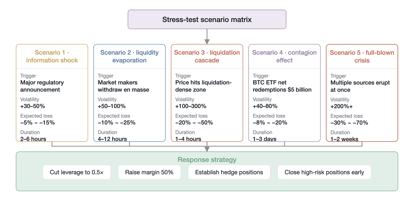
Figure 24-10. A four-source stress-test scenario matrix and response strategies (simulated-stress illustration, not measured data: the volatility, losses, and durations for each scenario are simulated magnitudes drawn from extreme events in crypto history, and the $5 billion net redemption from a BTC ETF is a hypothetical stress rather than a historical observation; data source: simulation parameters based on historical extreme events in crypto markets [49])
A core insight from the matrix is that the expected losses of the five scenarios do not grow linearly with the number of activated sources. Single-source scenarios usually cause manageable losses, because the other, unaffected market mechanisms can still provide a buffer; but when two or more volatility sources activate simultaneously, losses grow markedly superlinearly, owing to the interactive amplification among the volatility sources, and the expected loss of the full-crisis scenario may reach several to several dozen times that of a single-source scenario. In each scenario, the portfolio manager must measure three core metrics: the portfolio's overall expected loss, the position or asset that contributes most to the loss, and whether the remaining margin after the loss is sufficient—thereby identifying the portfolio's key vulnerabilities. The ultimate purpose of stress testing is not to predict when an extreme event will occur but to guide action: once the loss under a plausible scenario is unacceptable or would trigger cross-margin chain liquidations, the portfolio manager must reduce leverage, optimize holdings, or buy tail-hedging instruments before the scenario occurs, rather than reacting passively to depleted liquidity in a crisis. This forward-looking risk-control framework is a necessary condition for maintaining long-term operation in the perpetual futures market.
In practice, a portfolio manager should establish a systematic stress-testing process. First, the complete five-scenario stress test should be rerun at the end of each trading day, tracking the change in expected loss under each scenario. Second, when the market state machine transitions from one state to another, an additional stress test should be triggered immediately, because market structure is undergoing a qualitative change at that moment. Third, any newly added position or strategy must undergo an independent stress test before being incorporated into the portfolio, to assess its impact on overall portfolio risk under extreme scenarios. This continuous, multidimensional stress-testing framework can significantly improve a portfolio's resilience in a crisis and provides the portfolio manager with an objective, quantifiable basis for risk decisions. Beyond the forward scenario design above, reverse stress testing offers a complementary analytical perspective: instead of assuming a scenario and then computing the loss, it assumes an intolerable loss level (for example, 50% of total capital or the complete exhaustion of margin) and then works backward to infer what combination of market conditions would cause that loss. This approach helps uncover hidden vulnerabilities that forward scenarios miss. For example, reverse stress testing may reveal that certain seemingly diversified multi-asset portfolios in fact have highly concentrated risk exposure under a specific correlation-jump condition.
24.6 Applying volatility in systemic risk management
Volatility forecasting is a tool not only for micro-level traders and portfolio managers; it is equally a core input to the systemic risk management of cryptocurrency exchanges and decentralized derivatives protocols. In traditional risk-control frameworks, exchanges often rely on static parameters to manage risk, but in the perpetual futures market—which trades around the clock and carries extremely high leverage—static parameters cannot keep pace with rapid transitions in the volatility state. This section explores how to embed volatility-forecasting signals in the underlying architecture of exchanges and protocols, from dynamic margin calibration, to sensitivity adjustment of liquidation parameters, to a multi-tier liquidity early-warning system, ultimately building a volatility-driven real-time monitoring loop.
24.6.1 Dynamic margin calibration
In current perpetual futures market practice, most exchanges and protocols use a fixed maintenance margin rate. Although mainstream exchanges have adopted a tiered margin system based on position size (for example, Binance's maintenance margin rate for BTC perpetual futures rises in tiers from 0.4% to 5% with notional position size), the margin rate still does not adjust in real time to the market's volatility state [50]. This static design maximizes capital efficiency during calm periods, but when volatility rises sharply, a fixed margin rate cannot provide enough buffer, leaving the liquidation engine facing a substantial risk of accounts breaching into negative equity.
The core logic of a dynamic margin design is to establish a functional relationship between the margin rate and forecast volatility. When the system forecasts that future volatility will rise significantly, the exchange proactively raises margin requirements, forcing highly leveraged traders to reduce leverage or add margin before systemic risk accumulates. From the standpoint of statistical calibration, given the volatility forecast for a specific time window, the maintenance margin rate should be set so that, within a specified confidence interval, an extreme price move will not drive position equity below zero [51]. This mechanism ties micro-level margin requirements directly to macro-level volatility expectations.
Such dynamic calibration is not merely a mathematical tool of risk management but a concrete implementation of the "prevention layer" mechanism in protocol governance (as discussed in Section 21.2.2). When the volatility-forecasting model indicates an imminent high-volatility state, dynamically raising margin in effect transmits a risk signal to the market, suppressing speculative position-building by raising the cost of capital. Research shows that treating crypto assets as an independent risk class and calibrating margin according to their distinctive volatility characteristics can significantly reduce the probability of systemic default [52].
The dynamic margin mechanism, however, itself harbors a procyclicality risk that cannot be ignored. Raising margin requirements when volatility rises forces under-margined traders to close positions, and this concentrated closing itself pushes volatility higher, forming a positive feedback loop—precisely the margin-level counterpart of the model-homogeneity problem discussed in Section 24.7.2. Traditional financial regulatory frameworks have proposed systematic responses to this problem: Basel III's countercyclical capital buffer requires banks to accumulate extra capital during booms to meet demand during downturns, and the CPMI-IOSCO central counterparty (CCP) margin standards explicitly require central counterparties to incorporate anti-procyclicality mechanisms into their margin models. Dynamic margin design in crypto markets can draw on this experience—for example, by setting a speed cap on margin increases to avoid violent adjustments over a short interval, or by pre-collecting a "countercyclical margin add-on" during low-volatility periods to reduce the size of margin calls in high-volatility periods. In addition, dynamic margin faces challenges on the compliance front: in traditional finance, margin changes usually require advance notice to traders (CME, for example, gives one trading day's notice), and a crypto exchange that raises margin in real time without prior notice may face legal challenges regarding users' right to be informed, especially under emerging regulatory frameworks such as MiCA.
24.6.2 Adjusting liquidation parameters
The parameter settings of the liquidation engine directly determine the market's survivability in extreme conditions. In crypto derivatives markets, liquidation is usually benchmarked to the mark price rather than the last traded price, to prevent malicious manipulation caused by a short-term absence of liquidity [53]. The mark price is usually computed by combining the spot index price with a funding-rate basis component, and platforms differ in the specific method: Binance uses a moving average of the spot index plus basis, Hyperliquid uses a weighted median price, and dYdX v4 uses a multi-source median. Regardless of the specific method, the mark price always contains some form of smoothing parameter, and the fixity of this parameter in a high-volatility environment can become a source of systemic risk.
In a high-volatility environment, a longer smoothing window causes the mark price to lag severely behind the spot price. This lag not only provides arbitrageurs with risk-free attack exposure but, more dangerously, triggers an accumulation-release effect (see Section 22.4.3). When the lagging mark price finally catches up with the spot price, liquidation orders that should have triggered dispersed across different price levels are instead triggered simultaneously within an extremely short window, detonating a liquidation cascade [54].
Simply shortening the smoothing window, however, is also risky: it significantly increases the probability of noise liquidations, causing normal small price fluctuations to trigger unnecessary forced liquidations. Here the volatility-forecasting model provides a dynamic benchmark for resolving this trade-off: in the calm state, the system maintains a longer window to filter noise; when the volatility forecast rises sharply, the system automatically shortens the window to improve the mark price's responsiveness. This volatility-sensitive parameter-adjustment mechanism lets the liquidation engine strike a dynamic balance between smoothness and responsiveness. Dynamic parameter adjustment can, however, itself become an attack vector: an attacker who can predict the timing and direction of a parameter switch can profit from the change in liquidation rules at the moment it occurs. Parameter adjustment should therefore use gradual, continuous change rather than discrete jumps, so as to reduce the exploitable time window.
24.6.3 Liquidity early-warning systems
A more advanced form of embedding volatility signals in systemic risk management is to build a multi-tier liquidity early-warning system. Based on the five-stage liquidity model proposed in Chapter 20, an exchange can design an automated response mechanism spanning from a micro-trigger to a liquidation cascade. When a crisis erupts, human decision-makers often cannot keep pace with the execution speed of algorithmic trading, so the warning system's action responses must be highly automated.
Figure 24-11 uses a flowchart to show the three-tier response architecture of this liquidity early-warning system—tier-one micro-trigger detection, tier-two liquidity-ebb response, and tier-three liquidation-cascade emergency intervention—with each tier corresponding to progressively stricter trigger conditions and increasingly forceful risk-control measures.
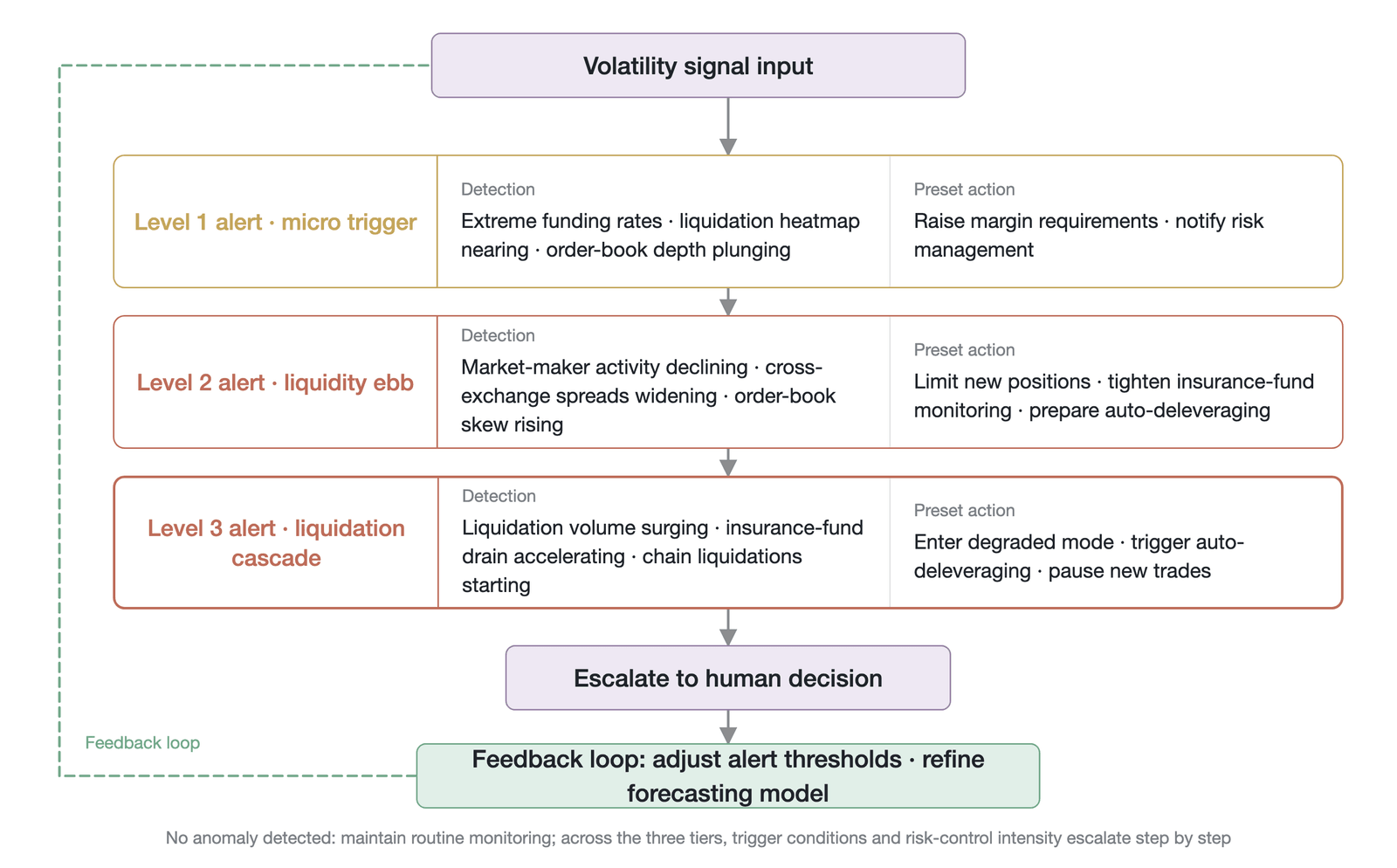
Figure 24-11. A flowchart of a volatility-signal-based liquidity early-warning and automated response system (structural illustration, not measured data; data source: an abstract construction of a protocol risk-management framework [55])
The key design feature of the architecture in the figure is that each warning tier pairs a "trigger condition" with a "preset action," and the mapping between the two is fixed in advance and executes automatically, without human intervention. Tier one is micro-trigger detection: triggered when a signal of surging volatility resonates with the proximity of a liquidation heatmap, its preset actions include raising the initial margin for new positions and sending a liquidity-demand signal to market makers. Research shows that such early turning points usually appear days or hours before violent market swings, providing an ample time window for proactive intervention [55].
If order book depth drops sharply and market makers' quote frequency declines markedly, the system escalates to tier two (liquidity ebb), taking more forceful measures such as restricting new positions in high-risk contracts and raising the maintenance margin rate. When liquidation volume grows exponentially and insurance-fund depletion breaches a safety threshold, the system enters tier three (liquidation cascade), and the protocol must automatically initiate a degradation mode—including suspending trading or activating auto-deleveraging (ADL)—to sever the positive feedback loop between falling prices and forced liquidations [56].
Implementing the warning and degradation mechanisms above faces fundamentally different governance challenges at centralized exchanges and decentralized protocols. A centralized exchange can have its risk-control team make an immediate decision to suspend trading—fast in response but opaque in process; a decentralized protocol's parameter adjustments usually require a governance process such as a multisig or a DAO vote, which simply cannot respond within the few minutes of a crisis. Concentrating the suspension authority in a single admin key, however, introduces a centralized single point of failure and a trust assumption. Both Hyperliquid's JELLY incident of 2025 and the Mango Markets incident of 2023 exposed this governance dilemma: the former was ultimately resolved through an emergency validator vote, while the latter was handled only retroactively through a governance process after the attack had occurred. Decentralized protocols must find a balance between response speed and decision legitimacy—for example, by using pre-authorized automated risk parameters (which trigger automatically under preset conditions, without a real-time vote) to ease this tension.
In addition, the calibration of warning thresholds is itself an ongoing practical challenge. If thresholds are set too sensitively, they generate too many tier-one warnings, and the system and its users gradually grow immune to the warning signals (the "crying wolf" effect); if set too insensitively, warnings may arrive only after the crisis has already erupted. In practice, the thresholds themselves must also be adjusted dynamically as the market's baseline volatility level and structure change, creating a second-order "calibration of the warning system" problem.
24.6.4 The volatility dashboard
To put the risk-control logic above into practice, exchanges and large protocols need a real-time monitoring framework that integrates all the underlying signals. This system, called the "volatility dashboard," not only aggregates forecast data from different sources but also serves as the hub connecting signals to automated decisions.
Figure 24-12 shows the conceptual design of this volatility dashboard, arranging five core monitoring panels in logical order from micro to macro, with each panel corresponding to an independent risk dimension while achieving cross-panel correlation through an underlying data pipeline.
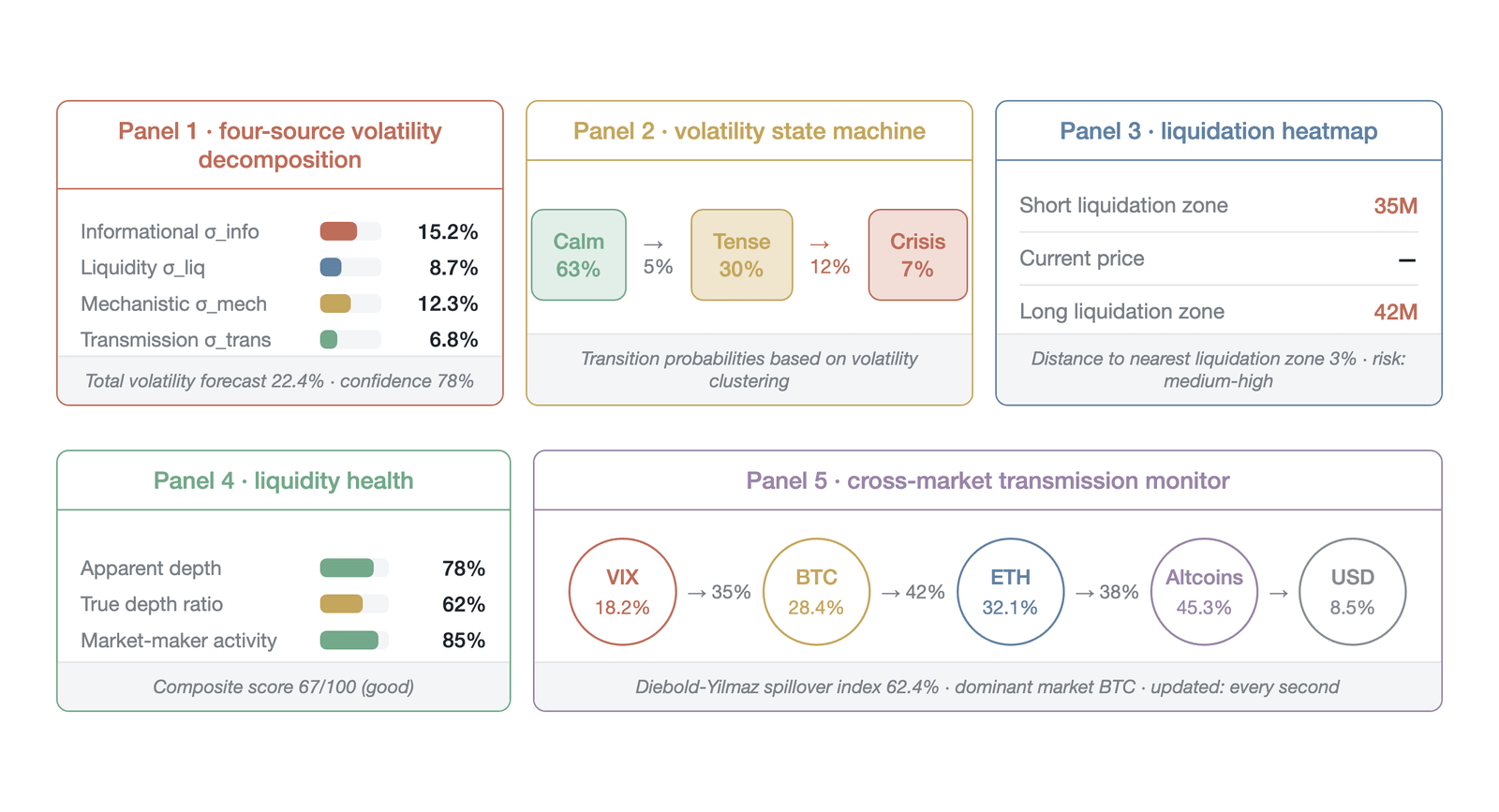
Figure 24-12. The conceptual design of a volatility dashboard and its real-time monitoring panels (conceptual-design illustration: the panel values are representative examples, not a measured snapshot; the variance sum of the four source components is approximately 22.4%, consistent with the conventions of the main text; data source: the author's design based on financial risk-monitoring architecture)
The dashboard's design follows the principle of "single view, multidimensional drill-down": on one interface, risk-control personnel can simultaneously observe the real-time decomposition of four-source volatility, the transition probabilities of the state machine, the spatial distribution of the liquidation heatmap, liquidity health, and cross-market transmission strength. The interconnection among these five panels is the core value of the system. For example, when panel one shows a sharp rise in estimated mechanical volatility, panel three simultaneously shows a narrowing distance to a liquidation cluster, and panel four confirms that liquidity depth is falling, the resonance of the three automatically triggers an escalated response from the warning system. This monitoring framework closes the full loop—from signal collection, to warning triggering, to execution of preset actions, to feedback adjustment—and is where systemic risk management in the perpetual futures market finally takes concrete form.
24.7 The limits of volatility forecasting
Understanding the limits of forecasting capability is an indispensable part of volatility modeling. Volatility forecasting is an effective tool, but over-reliance on models leads to an accumulation of model risk. This section systematically reviews the inherent limitations of volatility forecasting to help the reader develop a healthy skepticism toward models and avoid treating forecast outputs as certainties. Effective risk control is not about predicting everything but about modeling the predictable part and defending against the unpredictable part.
24.7.1 The decay of predictability
The capability of volatility forecasting does not extend linearly over time but has a clear physical boundary. Within this boundary, market microstructure and historical data provide rich information; beyond it, a forecasting model's effectiveness rapidly decays to no better than a random walk. The speed and degree of this decay are the core metric for evaluating the practical value of any volatility model.
Short-term (one to four hours) realized volatility is highly predictable. This predictive power comes mainly from the clustering effect of volatility—periods of high volatility tend to be followed by periods of high volatility. As earlier chapters discussed, the state-machine model provides powerful medium-term conditional forecasting capability by identifying the market's calm, stressed, or crisis state. In addition, intraday and intra-week periodic patterns, as well as the periodic pulse of funding settlement, all provide highly deterministic inputs for short-term forecasting. When the price approaches a liquidation cluster, the conditional probability of a rise in volatility can be computed precisely from the liquidation heatmap, which is the most valuable forecast of tail risk.
When the forecast horizon exceeds one to two days, however, a half-life effect on information begins to appear. The classic study by Engle and Patton (2001) [57] shows that volatility is highly persistent, with markedly different characterizations of persistence across model specifications—their estimate of the half-life of market volatility is about 73 days. This divergence itself reflects a deeper problem: our understanding of volatility dynamics is far from mature. In cryptocurrency markets, this decay is even more severe. The empirical study of cryptocurrency volatility forecasting by Ftiti et al. (2021) [58] shows that the predictive power of every class of volatility model decays rapidly as the forecast horizon lengthens, with forecast accuracy falling sharply beyond the short-to-medium term. This finding has major implications for risk control in the perpetual futures market: position-sizing decisions that rely on multi-day volatility forecasts lack sufficient statistical support, and their forecast errors exceed the precision acceptable for risk management.
Figure 24-13 depicts the complete trajectory along which the forecasting power (measured by R² or the correlation coefficient) of different types of volatility-forecasting models decays as the forecast horizon lengthens. This decay curve is the most intuitive tool for understanding the practical boundary of volatility forecasting.
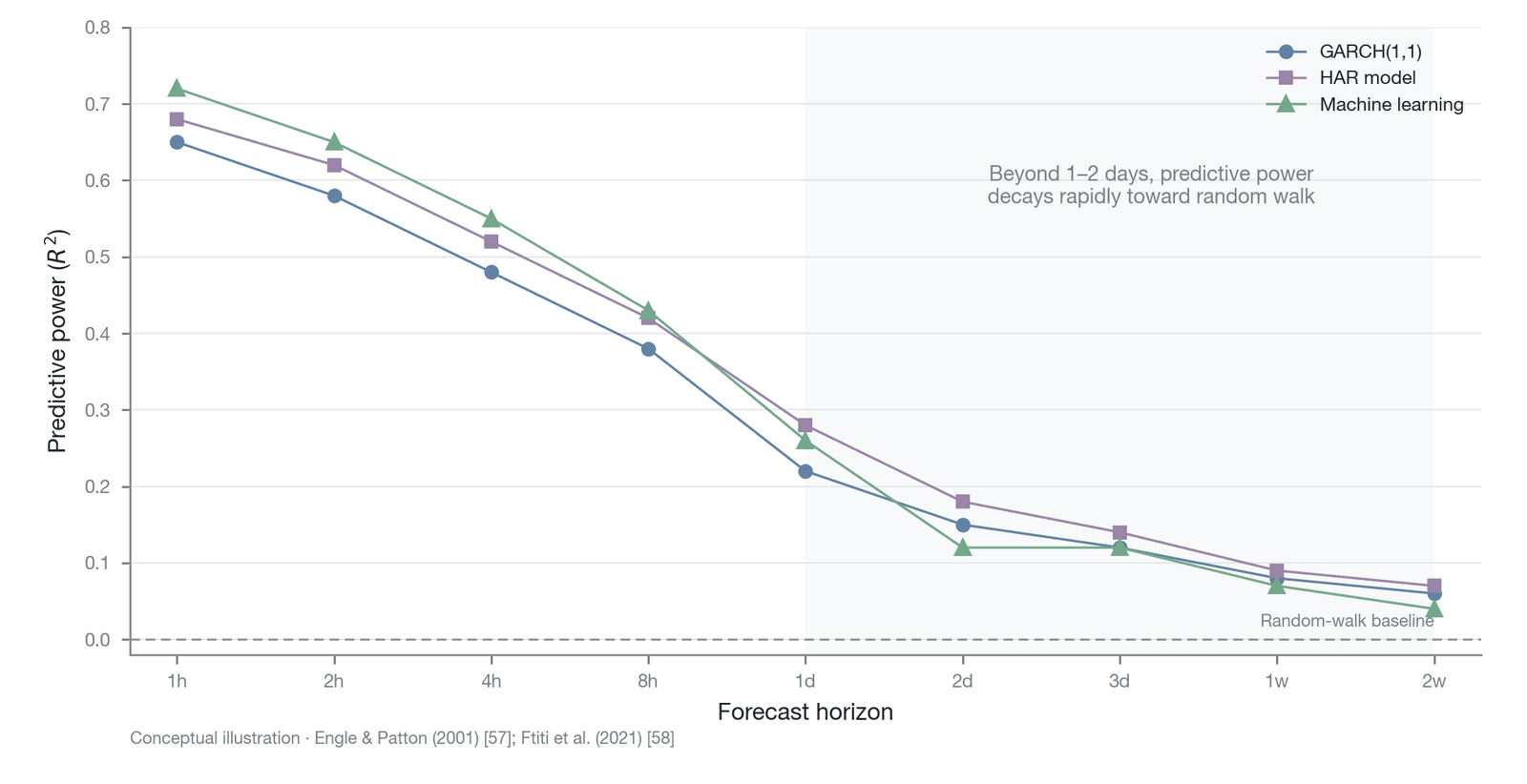
Figure 24-13. The decay curve of volatility-forecasting power over the forecast horizon (conceptual depiction, not measured data: the R² magnitudes and the shape of the decay are anchored to the empirical findings of Engle & Patton 2001 [57] and Ftiti et al. 2021 [58], and the claim that predictability approaches a random walk beyond one to two days is a qualitative conclusion; this figure depicts the decay of forecast R² over the forecast horizon, a distinct concept from the roughly 73-day half-life of volatility persistence in [57])
The most striking feature in the figure is the nonlinear shape of the decay curve. Within the short-term window (one to four hours), every class of model maintains relatively high forecast accuracy and the curve declines gently; but in the critical region of one to two days, the curve exhibits a sharp "cliff," with forecasting power collapsing dramatically over a very short interval. In cryptocurrency markets, this cliff is steeper than in traditional financial markets, reflecting their faster structural change and shorter information half-life. Beyond the cliff the curve flattens, the differences in forecasting power among the classes of model disappear, and all approach a random walk. The implication for risk-control practice is clear: volatility forecasts beyond two days are statistically unreliable, and position decisions based on such long-term forecasts lack adequate support. Especially difficult to predict is volatility driven by sudden events—true "news" such as a regulatory raid or the bankruptcy of a large exchange—whose timing is intrinsically impossible to infer from any known signal; and market-institutional changes such as the entry and exit of new market makers, the launch of new types of derivatives, or shifts in regulatory policy fundamentally alter the underlying structure of volatility. Even when a liquidity crisis's vulnerability can be identified from the liquidation heatmap, its exact trigger point and the subsequent nonlinear evolution path lie beyond the forecasting capability of statistical models, because extreme events often involve a qualitative rather than a quantitative change in participants' behavior.
24.7.2 Model-homogeneity risk
When most participants in the market use similar volatility-forecasting models, the models themselves become a source of risk. This phenomenon, the accumulation of "model risk," reveals a deep paradox in modern quantitative finance: rational risk management at the individual level may, at the macro level, lead to systemic irrational collapse. The root of this paradox is that participants' behavior is not independent but is tightly coupled through market mechanisms.
Model homogeneity leads to synchronization of collective behavior. When the market experiences a slight anomaly, highly similar forecasting models issue "high-volatility warning" signals to their respective users at the same time. Participants receiving these signals make rational individual responses: market makers widen the bid-ask spread to protect inventory, directional traders reduce positions to control risk, and exchanges' risk-control systems automatically raise margin requirements. These behaviors are robust risk-control measures under normal conditions, but when they occur synchronously, driven by homogeneous signals, they trigger a systemic liquidity dry-up.
Figure 24-14 uses a cyclical flowchart to depict how model homogeneity, through the positive feedback loop of "model warning → synchronized withdrawal → liquidity dry-up → volatility spike → renewed model warning," amplifies a tiny initial disturbance into a systemic liquidity crisis.
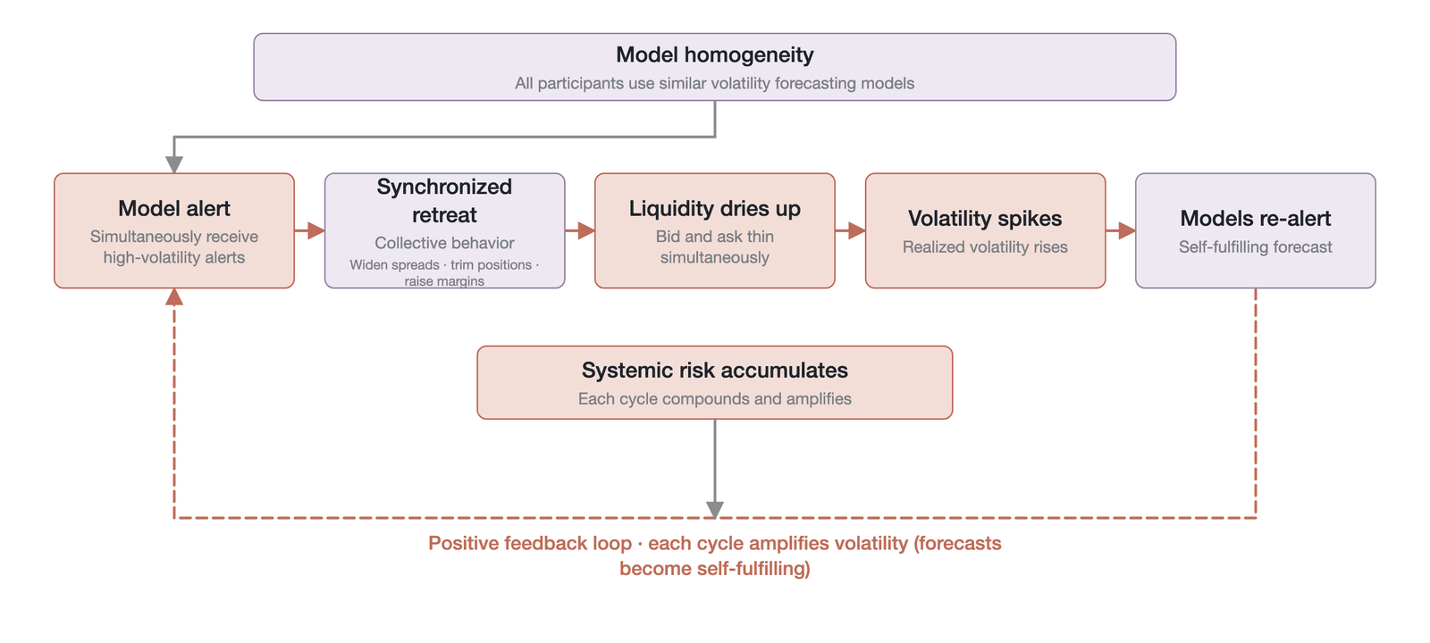
Figure 24-14. The accumulation of systemic risk triggered by the homogeneity of volatility-forecasting models (structural illustration, not measured data: a closed positive-feedback loop; the empirical anchor for the October 2025 cascade of roughly $19 billion in notional liquidations is given in the main text [60]; data source: compiled by the author)
The key node in the positive feedback loop shown in the figure is the step "volatility spike → renewed model warning": the rise in volatility induced by synchronized withdrawal is itself a product of deteriorating market microstructure, not a genuine fundamental information shock, but homogeneous forecasting models cannot distinguish the two and simply feed the higher volatility data into the next round of computation, outputting a higher-level warning signal. This synchronized withdrawal directly causes market liquidity to evaporate suddenly. The absence of liquidity means that even normal trading demand generates enormous price slippage, which further pushes up the actually observed volatility. This higher volatility data is then fed back into the forecasting models, triggering a new round of higher-level warnings. This positive feedback loop turns the models' forecasts into a self-fulfilling process through the synchronized behavior of participants. In traditional financial markets, in the Flash Crash of May 6, 2010, the homogeneous responses of algorithmic trading systems greatly worsened the market collapse, causing the S&P 500 index to fall by more than 5% within about 15 minutes and the Dow Jones Industrial Average to briefly plunge nearly 1,000 points [59].
In cryptocurrency markets, this homogeneity risk manifests even more extremely. Ali (2025) [60] dissects the October 2025 liquidation cascade and shows that similar risk-control parameter settings and automated liquidation programs triggered roughly $19 billion in liquidations (notional liquidation scale, not wiped-out open interest or actual losses) within about 36 hours. This liquidation cascade was characterized by a self-reinforcing spiral once triggered: the initial liquidation triggered a price drop, the drop set off more liquidations, and the additional liquidations further worsened the drop. Throughout this process, all exchanges and risk-control systems using the same liquidation trigger conditions executed the same operations at the same time, so that liquidity vanished entirely and price gaps became the norm.
The fundamental cause of model homogeneity is the concentration of "best practice" in the market. When a particular volatility-forecasting method is recognized by academia or industry as the "standard," all rational participants have an incentive to adopt it. This produces a "competitive convergence" in which most participants ultimately use the same or highly similar models. This convergence is itself harmless—even efficient—until the market faces a situation outside the models' assumptions. At that point, the homogeneous models fail simultaneously, producing systemic risk.
In crypto markets, model homogeneity has an additional, behavioral source that goes beyond the rational-choice framework: the concentration of information sources. When large numbers of traders follow the same social-media volatility-warning accounts, the same liquidation-data dashboards, or the same on-chain analytics platforms, the synchronization of their behavior comes not only from the similarity of the models themselves but also from the resonance of information inputs and narrative frames. This information-concentration-driven behavioral synchronization also exists in traditional financial markets (such as reliance on the Bloomberg terminal and on the same set of analyst reports), but in crypto markets it is further amplified by the instantaneous transmission effect of social media. Looking ahead, as AI-agent trading spreads, if these agents are based on similar model architectures and training data, model homogeneity may reach an unprecedented magnitude, creating an "algorithmic monoculture" risk in which all agents produce almost identical outputs when facing the same inputs, and the system's diversity defense is completely dismantled.
The paths to mitigating model-homogeneity risk can be developed at three levels. At the individual level, participants can deliberately introduce a heterogeneous mix of models—for example, combining a statistical time-series GARCH model with a machine-learning-based nonparametric model, or incorporating contrarian indicators into the model inputs (such as a contrarian volatility signal: when most models forecast falling volatility, deliberately retaining a certain share of high-volatility estimates as a hedge). At the market level, large market makers and institutions can design asynchronous risk-control triggers, avoiding a situation in which all participants execute the same operation at exactly the same threshold. At the protocol level, decentralized derivatives protocols can consider introducing asynchronous liquidation triggers—for example, setting slightly different liquidation trigger conditions or time delays for positions of different sizes—so as to structurally break the positive feedback loop of synchronized liquidation. Although these measures cannot completely eliminate model-homogeneity risk, they can significantly reduce the probability of a systemic liquidity dry-up caused by synchronized behavior.
24.7.3 Overfitting and out-of-sample failure
A model that shines in backtesting but fails in live trading is a characteristic hazard of volatility forecasting: strong historical fit often gives way to mediocre—or even loss-making—out-of-sample performance. The core cause is overfitting: the model learns not only the true regularities in the data but also memorizes historical noise.
Overfitting is especially severe in cryptocurrency markets. The history of the perpetual futures market is relatively short, the data sample is limited, and samples of extreme events are especially rare. When researchers use high-dimensional machine-learning models with hundreds of features, the algorithm inevitably overfits these rare extreme events. Moreover, multiple-testing bias further worsens the problem. Researchers usually test hundreds or thousands of parameter combinations and select the best-performing one, ignoring the risk of statistical invalidity introduced by this selection process itself. López de Prado (2018) [61] points out that without appropriate correction for multiple-hypothesis testing, backtest results often severely overstate true predictive power.
A deeper cause lies in the continual evolution of market structure. The entry of new participant types (such as institutional investors or AI agents), the launch of new types of derivatives, and changes in regulatory policy all continually alter the data-generating process, causing models trained on past data to fail in the future. As discussed in Section 24.2.4, the "half-life" of an effective volatility-forecasting model in the perpetual futures market may be only 3 to 6 months; even a model that performs perfectly on the past two years of data cannot be guaranteed to remain effective over the next two months.
Practical recommendations for coping with overfitting include rigorous out-of-sample validation and time-series cross-validation. Keeping the model simple is another key principle: following Occam's razor, it is better to use a simple model that is slightly less accurate but robust than to rely on a complex black box that is perfect in backtesting but fragile in live trading. In addition, one should not over-rely on any single model; a combination of models with different underlying assumptions usually provides more robust forecasts. Finally, backtest results should be systematically discounted, assuming that live performance will be 20% to 50% lower than the backtest result—a conservative practice, but one that avoids major losses caused by overconfidence.
24.7.4 Black swan events
Extreme events, or "black swans," are by their nature events beyond the historical distribution and beyond the cognitive range of existing models. Any volatility-forecasting model calibrated entirely on historical data is, by definition, unable to predict the occurrence of such events. Attempting to use a statistical model to predict the timing and specific form of such events is methodologically infeasible, and such attempts produce a false sense of security that reduces the risk-management system's actual defense against extreme events.
Volatility-forecasting models fail in specific ways during extreme events. GARCH-family models assume that volatility evolves continuously and cannot capture the price jumps triggered by liquidation cascades (as discussed in Section 24.2.2). Liao (2013) [62] points out that if jumps are not modeled explicitly, the value of traditional realized-volatility models in risk management is greatly diminished. In the perpetual futures market, price jumps caused by liquidation cascades are a common phenomenon rather than a rare event, which casts serious doubt on the applicability of the standard GARCH model in this market.
Likewise, VaR models based on historical simulation severely underestimate risk during extreme events, because the current tail event may be more extreme than anything recorded in the historical sample. Daníelsson et al. (2013) [63] give a rigorous characterization of the subadditivity condition for VaR under multivariate fat-tailed distributions, showing that the reliability of tail-risk measures depends heavily on the assumptions about the distribution's tails: once the actual tail is fatter than the model assumes, standard methods easily distort the characterization of extreme losses. This means that even a risk model that has performed well over the past decade cannot be guaranteed to correctly estimate risk under extreme market stress.
More deceptive still is the "calm trap." On the eve of many black swan events, the market often maintains a low volatility level, and all forecasting models show risk at a historical low. This false sense of security prompts participants to increase leverage, thereby accumulating structural fragility for the subsequent market collapse. This mechanism has a deep structural correspondence with Minsky's financial instability hypothesis: low volatility → low realized volatility → low margin consumption → traders increase leverage → systemic fragility accumulates → eventual collapse, which is precisely the crypto-market mapping of Minsky's "stability breeds instability." The quantitative study of systemic risk in cryptocurrency markets by Franco and Laurini (2025) [64] shows that systemic risk contagion often occurs within hours, and conventional daily risk metrics simply cannot provide a warning. In the FTX collapse of November 2022, BTC fell from about $21,000 to about $15,500 (a decline of more than 25%) over the three days from November 6 to November 9, and yet in the days before the event erupted the market still maintained a low volatility level, with no forecasting model having given an adequate warning.
Faced with this intrinsic unpredictability, the design of a risk-management system should acknowledge the limits of models' capability. Effective risk control is not about trying to predict all extreme events but about building systemic resilience to them. Constructing this resilience rests on two layers: the first is the statistical-model layer, used to optimize decisions under normal market states; the second is the rule-constraint layer, a set of hard risk-control rules that do not depend on model output, ensuring that the system can still maintain basic operation when the model fails.
Through rigorous position-size control, participants can ensure that the maximum loss on any single trade does not exceed a fixed proportion of total capital, for example 2%. This proportion must be adjusted for the leverage actually used in a high-leverage environment: at 10x leverage, a 2% capital loss corresponds to a roughly 0.2% price move, still a reasonable stop-loss range; but at 50x leverage, the same capital loss corresponds to only a 0.04% price move, which can be triggered within seconds even under normal market conditions, rendering the stop-loss rule useless. Through firm stop-loss discipline, a trader can close a position immediately once the loss reaches a preset level, avoiding a further widening of the loss. Through an ample liquidity reserve, exchanges and risk-control systems can maintain operational capacity during extreme events rather than being forced to liquidate at extreme prices. None of these measures aims to predict a black swan; they aim to ensure that, when a black swan inevitably appears, losses are bearable rather than unbearable.
Volatility can be studied and partly predicted, but its inherent randomness cannot be completely eliminated. Understanding the sources, dynamics, and predictability boundaries of volatility can improve the quality of risk-management decisions, but it cannot eliminate all uncertainty. A clear-eyed recognition of the limits of models' capability, and a tail-risk budgeting mechanism based on that recognition, are the prerequisites for volatility forecasting to deliver value in practice.
24.8 Chapter summary
In the perpetual futures ecosystem, which lacks a deep options market, participants face a core challenge: how to sense and forecast volatility risk without the benchmark of implied volatility. This chapter has built a complete closed-loop framework running from knowledge of volatility, to forecasting, to decision-making, turning the theoretical insights of the previous two chapters into operational tools. The starting point of this framework is to identify the set of alternative volatility signals specific to perpetual futures, including the degree of extremity of the funding rate, the spatial distribution of open interest in the liquidation heatmap, leading changes in order book depth, and cross-exchange spread anomalies [65]. Although these signals are limited in any single dimension, a reasonable combination of them can effectively capture volatility risk from different sources.
Based on this signal set, the chapter proposed a source-decomposed volatility forecasting method. Traditional unified modeling tries to capture total volatility with a single econometric model, but often performs poorly in the face of the extreme jumps of liquidation cascades and the periodic pulses of funding settlement [66]. The source-decomposed framework, by contrast, models informational, liquidity, mechanical, and transmission volatility separately and then aggregates them, fully exploiting the differences among the sources in time scale and predictability. Its core advantage is interpretability: when the forecast shows a rise in volatility, the risk manager can accurately judge the driving source (informational, liquidity, mechanical, or transmission) and respond in a targeted way.
The ultimate purpose of moving from signal to forecast is to guide decisions. The chapter embedded the forecast outputs in the micro- and macro-level decision processes of different market participants, forming a three-layer decision architecture. At the micro layer, market makers dynamically adjust their quoting strategy based on real-time identification of the volatility state; at the meso layer, portfolio managers use volatility-adjusted position sizing and the CVaR model to manage directional exposure; at the macro layer, exchanges and protocol designers guard against systemic risk through volatility-sensitive dynamic margin mechanisms and liquidity early-warning systems [60]. The core innovation of this closed-loop framework is that it provides not only a tool for measuring risk but also a set of conditional action rules based on the volatility state.
The framework established in this chapter has three key improvements over volatility analysis in traditional finance. First, it explicitly acknowledges the distinctive phenomenon of mechanical volatility in the perpetual futures market—volatility created out of nothing by liquidation cascades and the funding-settlement mechanism, rather than arising from information arrival or liquidity changes. Second, it exploits the special data advantages of perpetual futures, including real-time liquidation heatmaps, funding-settlement schedules, and order book microstructure—data that are hard to obtain in traditional futures markets. Third, it combines volatility forecasting with the specific incentive structures of market participants rather than remaining at the level of abstract risk measurement.
Different types of market participant draw different tools from this framework. Market makers rely on volatility-state identification to achieve dynamic spread adjustment and strategy-mode switching; their core competency is the real-time discrimination between liquidation-driven mechanical volatility and information-driven structural volatility, enabling a correct stay-or-withdraw decision during a sharp price drop. Directional traders and portfolio managers use source-decomposed forecasts for volatility-adjusted position sizing, proactively reducing the leverage multiple rather than merely shrinking the notional position when volatility is high, and identifying a portfolio's vulnerabilities in advance through stress-test scenario design based on the four-source theory [67]. Protocol designers and exchanges embed volatility forecasts in dynamic margin calibration and tiered liquidity early-warning systems, triggering a degradation mode before systemic risk accumulates. The output of the same volatility-forecasting model must be translated into three different decision signals, which requires the risk-management system to be highly flexible and modular in design.
Having built a complete framework from theory to practice, one must be clear about the epistemological boundary of this system: volatility forecasting is essentially a tool for reducing uncertainty, not a method for eliminating it. Intraday liquidity patterns, the periodic pulse of funding settlement, and the inertia effect of volatility clustering belong to the highly predictable category and usually account for 30% to 50% of total volatility. Sudden information shocks, extreme events, and the nonlinear evolution path after a liquidation cascade begins are intrinsically difficult to predict precisely [67]. A robust risk-management system must be built on the principle of modeling the predictable part and defending against the unpredictable part—even if the model forecasts that volatility will remain at 20%, the risk manager must still reserve an adequate capital buffer for the possibility that volatility suddenly jumps to 100%. In the perpetual futures market, the best risk managers are not those with the most complex forecasting models but those who maintain the clearest recognition of their own models' limitations and reserve an ample tail-risk budget accordingly.
As the final chapter of Part Eight, this chapter has not only completed a full account of volatility from its sources and dynamics to its forecasting and decision-making but has also laid the micro-level foundation for subsequent parts on market-quality assessment and the economics of regulation. Having understood the endogenous interaction between liquidity and volatility, the following analysis turns to a more macro perspective, exploring how these micro-level mechanisms shape the efficiency of price discovery across the whole market, and under what conditions external regulatory intervention must be introduced to correct market failures. The volatility-analysis framework established in this chapter will be used in subsequent parts to evaluate multiple dimensions of market quality, including the accuracy of price discovery, the reasonableness of transaction costs, and the controllability of systemic risk.
References
[1] Coinglass. (2024). Cryptocurrency derivatives market liquidation data. https://www.coinglass.com/LiquidationData
[2] Ho, T., & Stoll, H. R. (1981). Optimal dealer pricing under transactions and return uncertainty. Journal of Financial Economics, 9(1), 47–73. https://doi.org/10.1016/0304-405X(81)90020-9
[3] Engle, R. F., & Manganelli, S. (2004). CAViaR: Conditional autoregressive value at risk by regression quantiles. Journal of Business & Economic Statistics, 22(4), 367–381.
[4] Mathias, S. E., & Sahoo, S. (2025). Dynamic connectedness and systemic risk in global futures: Evidence from cryptocurrency, financial, and commodity markets. Eurasian Economic Review, 16(1), 311–350. https://doi.org/10.1007/s40822-025-00353-8
[5] Mandelbrot, B. B. (1963). The variation of certain speculative prices. The Journal of Business, 36(4), 394–419. https://doi.org/10.1086/294632
[6] Cont, R. (2007). Volatility clustering in financial markets: Empirical facts and agent-based models. In G. Teyssière & A. P. Kirman (Eds.), Long Memory in Economics (pp. 289–309). Springer.
[7] Mayhew, S. (1995). Implied volatility. Financial Analysts Journal, 51(4), 8–20.
[8] Mixon, S. (2009). Option markets and implied volatility: Past versus present. Journal of Financial Economics, 94(2), 171–191. https://doi.org/10.1016/j.jfineco.2008.09.010
[9] Ackerer, D., Hugonnier, J., & Jermann, U. J. (2025). Perpetual futures pricing. Mathematical Finance. Advance online publication. https://doi.org/10.1111/mafi.70018
[10] Zhivkov, P. (2026). The two-tiered structure of cryptocurrency funding rate markets. Mathematics, 14(2), 346. https://doi.org/10.3390/math14020346
[11] Gornall, W., Rinaldi, M., & Xiao, Y. (2024). Perpetual futures and basis risk: Evidence from cryptocurrency (Working Paper). SSRN.
[12] McGroarty, F., ap Gwilym, O., & Thomas, S. (2006). Microstructure effects, bid–ask spreads and volatility in the spot foreign exchange market pre and post-EMU. Global Finance Journal, 17(1), 23–49. https://doi.org/10.1016/j.gfj.2006.06.004
[13] Degryse, H., De Winne, R., Gresse, C., & Payne, R. (2020). Cross-venue liquidity provision: High frequency trading and ghost liquidity (ESMA Working Paper No. 4). European Securities and Markets Authority.
[14] Makarov, I., & Schoar, A. (2019). Price discovery in cryptocurrency markets. AEA Papers and Proceedings, 109, 97–99. https://doi.org/10.1257/pandp.20191020
[15] Chi, Y., Chu, Q., & Hao, W. (2024). Return and volatility forecasting using on-chain flows in cryptocurrency markets. arXiv preprint arXiv:2411.06327. https://doi.org/10.48550/arXiv.2411.06327
[16] Andersen, T. G., & Bollerslev, T. (1998). Answering the skeptics: Yes, standard volatility models do provide accurate forecasts. International Economic Review, 39(4), 885–905.
[17] Corsi, F. (2009). A simple approximate long-memory model of realized volatility. Journal of Financial Econometrics, 7(2), 174–196. https://doi.org/10.1093/jjfinec/nbp001
[18] Barndorff-Nielsen, O. E., & Shephard, N. (2004). Power and bipower variation with stochastic volatility and jumps. Journal of Financial Econometrics, 2(1), 1–37.
[19] Kim, J.-M., Jun, C., & Lee, J. (2021). Forecasting the volatility of the cryptocurrency market by GARCH and stochastic volatility. Mathematics, 9(14), 1614.
[20] Engle, R. F. (1982). Autoregressive conditional heteroscedasticity with estimates of the variance of United Kingdom inflation. Econometrica, 50(4), 987–1007. https://doi.org/10.2307/1912773
[21] Bollerslev, T. (1986). Generalized autoregressive conditional heteroskedasticity. Journal of Econometrics, 31(3), 307–327. https://doi.org/10.1016/0304-4076(86)90063-1
[22] Duan, J.-C., Ritchken, P. H., & Sun, Z. (2006). Jump starting GARCH: Pricing and hedging options with jumps in returns and volatilities (Working Paper No. 06-19). Federal Reserve Bank of Cleveland.
[23] Chen, K. S., & Yang, J. J. (2024). Price dynamics and volatility jumps in bitcoin options. Financial Innovation, 10(1), 132. https://doi.org/10.1186/s40854-024-00653-z
[24] Zhu, H., Bai, L., He, L., & Liu, Z. (2023). Forecasting realized volatility with machine learning: Panel data perspective. Journal of Empirical Finance, 73, 251–271.
[25] Corsi, F., Audrino, F., & Renò, R. (2012). HAR modeling for realized volatility forecasting. In L. Bauwens, C. Hafner, & S. Laurent (Eds.), Handbook of Volatility Models and Their Applications (pp. 363–382). Wiley.
[26] Kakade, K., Mishra, A. K., Ghate, K., & Gupta, S. (2022). Forecasting commodity market returns volatility: A hybrid ensemble learning GARCH-LSTM based approach. Intelligent Systems in Accounting, Finance and Management, 29(2), 103–117.
[27] Zhuo, Y., & Morimoto, T. (2024). A hybrid model for forecasting realized volatility based on heterogeneous autoregressive model and support vector regression. Risks, 12(1), 12.
[28] Mishra, A. K., Renganathan, J., & Gupta, A. (2024). Volatility forecasting and assessing risk of financial markets using multi-transformer neural network based architecture. Engineering Applications of Artificial Intelligence, 133, 108223. https://doi.org/10.1016/j.engappai.2024.108223
[29] Blanc, S. M., & Setzer, T. (2016). When to choose the simple average in forecast combination. Journal of Business Research, 69(10), 3951–3962. https://doi.org/10.1016/j.jbusres.2016.05.013
[30] Ben Omrane, W., Dabbou, H., Saadi, S., Savaser, T., & Sebai, S. (2025). Exploring volatility reactions in cryptocurrency markets using intraday macroeconomic news analysis. International Review of Economics & Finance, 103, 104509. https://doi.org/10.1016/j.iref.2025.104509
[31] Easley, D., López de Prado, M. M., & O'Hara, M. (2012). Flow toxicity and liquidity in a high-frequency world. The Review of Financial Studies, 25(5), 1457–1493. https://doi.org/10.1093/rfs/hhs053
[32] Hansen, P. R., Kim, C., & Kimbrough, W. (2024). Periodicity in cryptocurrency volatility and liquidity. Journal of Financial Econometrics, 22(1), 224–251. https://doi.org/10.1093/jjfinec/nbac034
[33] Brauneis, A., & Sahiner, M. (2026). Crypto volatility forecasting: Mounting a HAR, sentiment, and machine learning horserace. Asia-Pacific Financial Markets, 33(1), 379–411. https://doi.org/10.1007/s10690-024-09510-6
[34] Shahrour, M. H., Lemand, R., & Mourey, M. (2025). Cross-market volatility dynamics in crypto and traditional financial instruments: Quantifying the spillover effect. The Journal of Risk Finance, 26(1), 1–21. https://doi.org/10.1108/jrf-07-2024-0185
[35] Wyart, M., Bouchaud, J.-P., Kockelkoren, J., Potters, M., & Vettorazzo, M. (2008). Relation between bid–ask spread, impact and volatility in order-driven markets. Quantitative Finance, 8(1), 41–57.
[36] Avellaneda, M., & Stoikov, S. (2008). High-frequency trading in a limit order book. Quantitative Finance, 8(3), 217–224. https://doi.org/10.1080/14697680701381228
[37] Kalimipalli, M., & Susmel, R. (2004). Regime-switching stochastic volatility and short-term interest rates. Journal of Empirical Finance, 11(3), 309–329. https://doi.org/10.1016/j.jempfin.2003.10.001
[38] Auh, J. K., & Cho, W. (2023). Liquidation cascade and anticipatory trading: Evidence from the structured equity product market. The Review of Asset Pricing Studies, 13(1), 53–98. https://doi.org/10.1093/rapstu/raac010
[39] Park, A. (2023). The conceptual flaws of decentralized automated market making. Management Science, 69(11), 6731–6751. https://doi.org/10.1287/mnsc.2021.02802
[40] Hyperliquid. (2025). Protocol vaults: Hyperliquidity Provider (HLP). https://hyperliquid.gitbook.io/hyperliquid-docs/hypercore/vaults/protocol-vaults
[41] Thorp, E. O. (1975). Portfolio choice and the Kelly criterion. In Stochastic Optimization Models in Finance (pp. 599–619). Academic Press.
[42] Hsieh, C. H., Barmish, B. R., & Gubner, J. A. (2018). At what frequency should the Kelly bettor bet? 2018 Annual American Control Conference (ACC), 5485–5490. https://doi.org/10.23919/ACC.2018.8431224
[43] Laureti, P., Medo, M., & Zhang, Y.-C. (2010). Analysis of Kelly-optimal portfolios. Quantitative Finance, 10(7), 689–697. https://doi.org/10.1080/14697680902991619
[44] Ahmed, R. R., Vveinhardt, J., Štreimikienė, D., Ghauri, S. P., & Ashraf, M. (2018). Stock returns, volatility and mean reversion in emerging and developed financial markets. Technological and Economic Development of Economy, 24(3), 1149–1177.
[45] Abken, P. A., & Nandi, S. (1996). Options and volatility. Economic Review (Federal Reserve Bank of Atlanta), 81(3–6), 21–35.
[46] Renault, E., & Touzi, N. (1996). Option hedging and implied volatilities in a stochastic volatility model. Mathematical Finance, 6(3), 279–302. https://doi.org/10.1111/j.1467-9965.1996.tb00117.x
[47] Huisman, R., Koedijk, K. G., & Pownall, R. A. (1998). VaR-x: Fat tails in financial risk management. Journal of Risk, 1(1), 47–61.
[48] Sarykalin, S., Serraino, G., & Uryasev, S. (2008). Value-at-risk vs. conditional value-at-risk in risk management and optimization. In State-of-the-Art Decision-Making Tools in the Information-Intensive Age (pp. 270–294). INFORMS.
[49] Likitratcharoen, D., Chudasring, P., Pinmanee, C., & Wiwattanalamphong, K. (2023). The efficiency of value-at-risk models during extreme market stress in cryptocurrencies. Sustainability, 15(5), 4395.
[50] TD Securities. (2025). Perpetual futures: The missing link in tokenized equities. https://www.tdsecurities.com/ca/en/tokenized-equities-missing-link-perps
[51] Gate.io. (2026). Cryptocurrency derivatives risk weights are independent, higher volatility requires higher margin. https://www.gate.com/news/detail/18744636
[52] Amirdjanova, A., Lynch, D., & Zheng, A. (2026). Initial margin for crypto currencies risks in uncleared markets (FEDS Working Paper No. 2026-009). Federal Reserve Board. https://www.federalreserve.gov/econres/feds/files/2026009pap.pdf
[53] Allen, F., & Carletti, E. (2008). Mark-to-market accounting and liquidity pricing. Journal of Accounting and Economics, 45(2–3), 358–378. https://doi.org/10.1016/j.jacceco.2007.02.005
[54] Soska, K., Dong, J. D., Khodaverdian, A., Zetlin-Jones, A., Routledge, B., & Christin, N. (2021). Towards understanding cryptocurrency derivatives: A case study of BitMEX. Proceedings of the Web Conference 2021, 3450–3459.
[55] Song, S., & Li, H. (2025). Can topological transitions in cryptocurrency systems serve as early warning signals for extreme fluctuations in traditional markets? Physica A: Statistical Mechanics and its Applications, 657, 130194. https://doi.org/10.1016/j.physa.2024.130194
[56] Qin, K., Ernstberger, J., Zhou, L., Jovanovic, P., & Gervais, A. (2023). Mitigating decentralized finance liquidations with reversible call options. In Financial Cryptography and Data Security (pp. 344–362). Springer.
[57] Engle, R. F., & Patton, A. J. (2001). What good is a volatility model? Quantitative Finance, 1(2), 237–245.
[58] Ftiti, Z., Louhichi, W., & Ben Ameur, H. (2021). Cryptocurrency volatility forecasting: What can we learn from the first wave of the COVID-19 outbreak? Annals of Operations Research, 330(1), 665–690. https://doi.org/10.1007/s10479-021-04116-x
[59] Kirilenko, A. A., Kyle, A. S., Samadi, M., & Tuzun, T. (2017). The Flash Crash: High-frequency trading in an electronic market. The Journal of Finance, 72(3), 967–998. https://doi.org/10.1111/jofi.12498
[60] Ali, Z. (2025). Anatomy of the Oct 10–11, 2025 crypto liquidation cascade: Macroeconomic triggers, market microstructure, and systemic risk lessons. SSRN Electronic Journal. https://papers.ssrn.com/sol3/papers.cfm?abstract_id=5611392 https://doi.org/10.2139/ssrn.5611392
[61] López de Prado, M. (2018). Advances in financial machine learning. Wiley.
[62] Liao, Y. (2013). The benefit of modeling jumps in realized volatility for risk prediction: Evidence from Chinese mainland stocks. Pacific-Basin Finance Journal, 23, 25–48. https://doi.org/10.1016/j.pacfin.2013.01.002
[63] Daníelsson, J., Jorgensen, B. N., Samorodnitsky, G., Sarma, M., & de Vries, C. G. (2013). Fat tails, VaR and subadditivity. Journal of Econometrics, 172(2), 283–291. https://doi.org/10.1016/j.jeconom.2012.08.011
[64] Franco, J. P. M., & Laurini, M. P. (2025). Quantifying systemic risk in cryptocurrency markets: A high-frequency approach. International Review of Economics & Finance, 102, 104214.
[65] Naimy, V., Haddad, O., Fernández-Avilés, G., & El Khoury, R. (2021). The predictive capacity of GARCH-type models in measuring the volatility of crypto and world currencies. PLoS ONE, 16(1), e0245904. https://doi.org/10.1371/journal.pone.0245904
[66] Silva, L., & Maciel, L. (2025). Cryptocurrency price returns volatility modeling and forecasting with GARCH models. RAUSP Management Journal, 60(1), 225–239. https://doi.org/10.1108/rausp-04-2023-0056
[67] Joshi, P. (2025). Regime-specific interdependencies in cryptocurrency markets: A high-frequency GMM-VAR approach. Data Science in Finance and Economics, 5(3), 419–439.