On March 12, 2020, the cryptocurrency market suffered one of the most violent single-day crashes in its history, a day that came to be known as Black Thursday [1]. Within just 24 hours, the price of Bitcoin fell by nearly 50%, plunging from about $7,900 to a low of $3,867 [2]. This macro shock, triggered by global panic over the COVID-19 pandemic, set off an unprecedented liquidation cascade of leveraged positions in the crypto derivatives market; on BitMEX alone, liquidations exceeded $700 million [3]. Yet amid this collapse, in which evaporating liquidity intertwined with panic selling, the funding rate mechanism of the derivatives market malfunctioned severely: the price of BitMEX's XBTUSD perpetual futures traded at one point at a discount of more than 10% to spot, and the funding rate touched an extreme level of −0.375% in a single period [4].
At that particular moment, the price of the perpetual futures had fallen far below the spot price—BitMEX's XBTUSD perpetual traded at one point more than $500 below spot—exhibiting an extreme negative basis [5]. According to the standard theoretical description of the funding rate mechanism, such a negative basis should trigger a negative funding rate, under which shorts pay longs, thereby incentivizing traders to buy the perpetual and pushing its price back toward spot value. Yet even after the rate had turned extremely negative, the price failed to converge. Arbitrageurs, unable to deposit funds into BitMEX because of congestion on the blockchain network, could not execute the arbitrage [5]; the forced sell orders generated by the liquidation cascade continued to depress the perpetual price, forming a positive feedback loop of "extreme rate → still no correction → widening basis." Under conditions of evaporating liquidity, the funding rate's anchoring mechanism nearly failed entirely.
This extreme anomaly raises three fundamental questions about the underlying mechanism of perpetual futures. Where does the anchoring force of the funding rate actually come from? Is it a passive mathematical formula for correcting the price spread, or the equilibrium outcome of a complex, friction-laden game among multiple participants? Building on this, why does a mechanism that has functioned well more than 90% of the time break down so severely at exactly the moment when the market most needs it to anchor prices? And taking the analysis together, does the extreme behavior of the funding rate itself encode a deeper signal about the market's leverage state and systemic fragility?
To answer these questions, this chapter moves beyond the surface-level description of a "negative feedback loop of algorithmic anchoring" and builds a systematic game-theoretic analytical framework. It uses a three-layer decomposition model to deconstruct the economic components of the funding rate, employs an anchoring strength spectrum to measure the effectiveness boundary of the anchoring mechanism across different market states, and constructs a three-layer game model to analyze the interaction structure among longs and shorts, arbitrageurs, and exchanges. It then examines how rate polarization positive feedback explains the mechanism that generates extremes, and finally advances the funding rate as state variable hypothesis, which repositions the funding rate from a passive market "output" to a "predictor" of future volatility and systemic risk. Across these five nested frameworks, the chapter builds a chain of reasoning from foundational concepts to frontier analysis, arguing that the funding rate is a core variable for understanding the microstructure and game dynamics of the crypto derivatives market.
10.1 Mechanisms and definitions
Before turning to the game-theoretic analysis, we need a clear and rigorous shared vocabulary. The three-price system of perpetual futures, the internal structure of the funding rate formula, and the parameter differences across exchanges together set the initial conditions and payoff structure for every game that follows. They determine the profit margin available to arbitrageurs, the holding cost borne by speculators, and the resilience of the entire system under extreme stress. Before analyzing participants' strategies, we must define the rules of the game precisely.
10.1.1 The three-price system
The ability of perpetual futures to operate independently, free from the constraint of a delivery date, rests on a three-price system. Each of the three serves a distinct function, and their interaction keeps the market running. Understanding the distinctions and connections among them is a prerequisite for grasping the funding rate mechanism.
The index price is the objective value benchmark for the entire system. It is typically computed as a volume-weighted average of the latest traded prices across several major global spot exchanges, such as Coinbase, Kraken, and Bitstamp [6]. The index price is designed to provide a global-consensus value that is difficult for any single entity or large trade to manipulate. To ensure its robustness, exchanges usually build multiple anomaly-detection mechanisms into the calculation: automatically discarding price sources that deviate excessively, excluding data from periods of liquidity drought, and dynamically adjusting weights. For example, when one spot exchange's quote deviates from the median of the others by more than a certain threshold, that exchange's weight is automatically reduced or even set to zero. This design makes the index price a relatively "exogenous" variable: it reflects the aggregate state of the global spot market rather than the internal supply-and-demand dynamics of any single derivatives exchange. However, the exogeneity assumption for the index price holds only if its constituent exchanges have sufficient liquidity depth. For mainstream assets such as BTC and ETH, the weighted average across many highly liquid exchanges makes manipulation extremely costly, so the exogeneity assumption holds reasonably well. For long-tail assets with low circulating market capitalization, however (such as ALPACA, analyzed later in this chapter), the constituent exchanges may be extremely thin, and a single medium-sized market order can move the spot price significantly and thereby affect the index price. At that point, the "exogenous anchor" assumption of the three-price system partly breaks down: a manipulator can influence both the index price and the perpetual price at once, fundamentally weakening the anchoring foundation of the rate mechanism. The Mango Markets exploit of October 2022 is a canonical case: the attacker, Avraham Eisenberg, manipulated the price of the MNGO token in a low-liquidity spot market, successfully affecting the oracle price feed and ultimately causing protocol losses of over $110 million (per CFTC and DOJ figures). This risk dimension is developed further in the analysis of funding-rate-manipulation feasibility in Section 10.6.3.
The perpetual price—the latest traded price on the derivatives order book—is a direct indicator that reflects, in real time, the internal supply and demand, leverage direction, and trading sentiment of the derivatives market. It forms directly through the bidding of longs and shorts within the exchange and is therefore highly "endogenous." When large numbers of leveraged longs pour in, the perpetual price is driven above the index price, forming a positive premium; conversely, when panic selling or short-side force dominates, the perpetual price falls below the index price, forming a negative premium (i.e., a discount). Yet precisely because of this endogeneity, the perpetual price is highly vulnerable to the impact of a single large order or short-term manipulation, and one sufficiently large market order can create a significant price deviation during a thinly traded period.
The mark price, in turn, is a design product that strikes a balance between anchoring to true value and reflecting market reality. It is typically composed of a robust index price plus a moving-averaged basis (the difference between the perpetual price and the index price) [7]. The mark price calculation differs fundamentally across exchanges: BitMEX uses a composite calculation based on the order-book mid-price and the index price, with an exponential moving average (EMA) window length that varies by contract; Binance takes a weighted average of the index price and the best-bid/best-ask mid-price, with weights that adjust dynamically to a contract's liquidity conditions; and Hyperliquid uses the oracle median price plus a small-window EMA basis. These differences directly determine the moment at which liquidation is triggered: under identical market conditions, the same trader may be liquidated on one exchange but not on another. The mark price serves two core functions. First, it is the sole basis for computing unrealized profit and loss (P&L) and assessing margin levels. Second, during extreme volatility it serves as the warning line that triggers forced liquidation. The mark price is designed to filter out short-term noise in the perpetual price, providing a buffer layer for the market. If the perpetual price were used directly to trigger liquidations, a brief wick—a sharp price deviation over a very short interval that quickly reverts—could unnecessarily liquidate large numbers of innocent positions. Through its smoothing mechanism, the mark price minimizes this risk.
The interaction among these three prices constitutes the infrastructure on which the funding rate operates: the basis, time-weighted and averaged, becomes the premium component that drives the rate calculation, while the mark price maintains the system's solvency floor, preventing over-leveraged positions from triggering systemic risk over transient price disturbances.
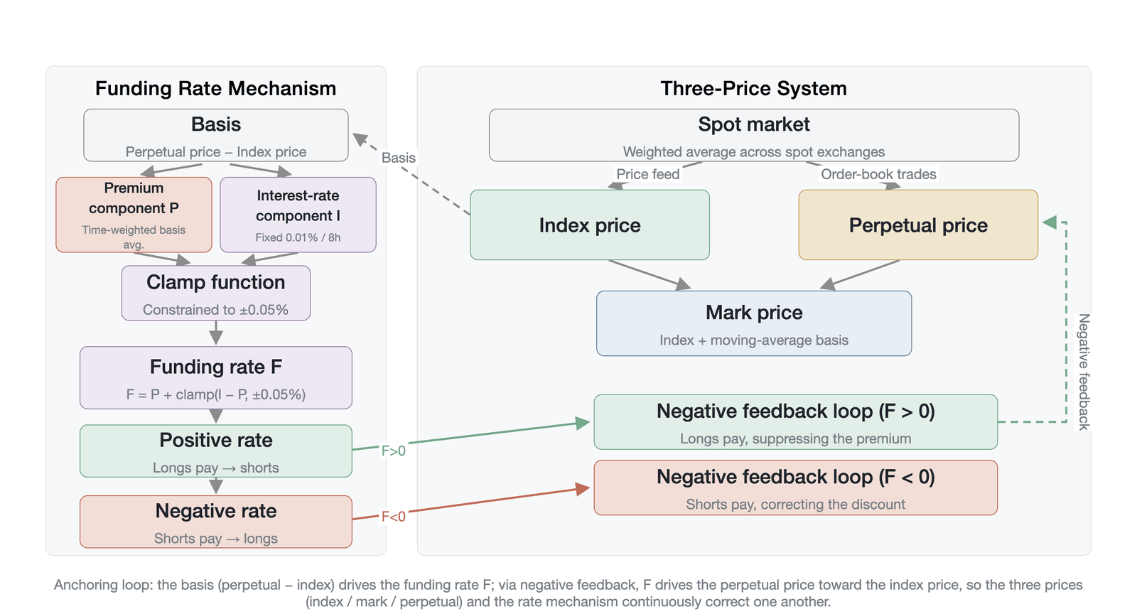
Figure 10-1. The three-price system of perpetual futures and the funding rate anchoring mechanism
10.1.2 Deconstructing the funding rate formula
The details of the funding rate calculation may vary slightly across exchanges, but the core logic is highly consistent. Taking the common formula used by major exchanges, the funding rate F can be deconstructed into the following form [8]:
where F is the funding rate, P is the premium component, and I is the interest rate component.
This formula carries several layers of economic meaning: the premium component captures the market's directional preference, the interest rate component embeds the capital cost of holding a position, and the clamp function introduces nonlinear institutional friction through its boundary constraints. Their interaction gives the funding rate markedly different response characteristics across market states: it is locked to a fixed baseline under mild deviations, and only under extreme deviations does it exhibit linear sensitivity to the premium.
The premium component is the most information-dense dynamic part of the rate, directly quantifying the degree to which the perpetual price deviates from the index price. It is usually the time-weighted average of the basis over a window (such as the 8-hour settlement period) rather than a simple instantaneous snapshot. Specifically, BitMEX uses a time-weighted average price (TWAP) over the past minute, Binance uses an arithmetic mean sampled every minute within the settlement period, and Hyperliquid uses an average over a 1-hour window of samples taken every 5 seconds. These sampling differences directly affect how sensitive the rate is to short-term price shocks. This time-weighting has a direct effect: it prevents traders from manipulating the rate by momentarily creating a large basis just before settlement, and it also makes the rate reflect a sustained directional preference over a period rather than transient noise. When P is positive, the perpetual has sustained a premium over the settlement period and long demand is strong; when P is negative, a sustained discount prevails and short-side force dominates. In short, the premium component prices the directional exposure that participants are willing to pay for, which makes it the most information-rich part of the rate.
The interest rate component reflects the capital cost of holding a synthetic leveraged position. When BitMEX pioneered perpetual futures in 2016, it set this component at a fixed 0.01% every 8 hours (approximately 10.95% simple annualized) [9]; the institutional rationale for this interest rate component—why it is not a precise macro risk-free rate, and how it was set as an institutional benchmark to incentivize arbitrageurs to provide liquidity—is discussed in the financing cost layer of Section 10.2.1. As perpetual futures were widely adopted by major exchanges worldwide, this 0.01% interest rate component became a de facto industry standard that profoundly shaped the structural characteristics of the entire market.
The clamp function is an often-underestimated part of the formula, and its influence extends far beyond what it appears to have on the surface. It is a boundary-constraint function that forces the value of (I − P) into the interval . Its mathematical definition is:
The clamp function does more than limit extreme fluctuations. It creates an asymmetric effect that forms the basis for understanding the structural characteristics of the funding rate. To see this intuitively, we can analyze the response curve of the funding rate F to the premium component P. When the interest rate component I = 0.01%, the entire response relationship exhibits a three-segment piecewise-linear character (Table 10-1):
| Range of premium component P | Value of clamp | Final rate F = P + clamp | Economic meaning |
|---|---|---|---|
| (upper bound) | , declining linearly with | Deep-discount zone: the rate falls as the discount deepens, but is always "held up" by the correction term | |
| (no clamping) | (constant) | Stable band: the clamp offsets fluctuations in , locking the rate | |
| (lower bound) | , rising linearly with | Deep-premium zone: the rate rises as the premium deepens, but is "slowed" by the correction term |
Table 10-1. The three-segment piecewise-linear response of the funding rate to the premium component (interest rate component I = 0.01%) (Data source: compiled by the author)
Empirical data confirm the effect of this design [8]: BitMEX's Q3 2025 report shows that the BTC perpetual rate was exactly equal to 0.01% for 78.19% of the time and the ETH rate for 87.52% of the time. This does not mean the market was continuously at equilibrium—the premium component P in fact fluctuated continuously—but rather reflects a "stability illusion" created by the clamp function. This stable band thereby gives the funding rate a built-in positive bias: even when the market is slightly in discount, longs must still pay shorts, constituting a non-negligible "institutional friction layer." The full argument for this structural positive bias—including the width of the stable band, the critical example at P = −0.03%, and data on the share of positive rates—is formalized in the "three-layer decomposition model" of Section 10.2, specifically in Section 10.2.3.
10.1.3 Cross-exchange parameter differences
The funding rate is not a single, unified standard but a design space with multiple parameters. Differences across exchanges in settlement frequency, the interest rate component, the clamp bounds, the composition of the index price, and rate caps may look like mere "technical implementation details" on the surface, but they significantly alter participants' cost-benefit structures and thereby shape markedly different game environments. Understanding these differences is key to understanding why the funding rate for the same asset can behave so differently across platforms.
Table 10-2 compares the core design parameters of three representative exchanges—BitMEX, Binance, and Hyperliquid—across five dimensions: settlement frequency, the interest rate component, the clamp range, the rate cap, and the source of the index price. These parameter differences directly determine the response speed of arbitrage capital on each platform, the feasible cost of a manipulation attack, and the magnitude of rate polarization during extreme conditions.
| Design dimension | BitMEX | Binance | Hyperliquid |
|---|---|---|---|
| Settlement frequency | Every 8 hours (fixed) | Dynamic (8h / 4h / 1h) [10] | Every 1 hour (fixed) [11] |
| Interest rate component | 0.01% / 8h | 0.01% / 8h | 0.01% / 8h (actual payment of per 1h) [11] |
| Clamp range | ±0.05% | ±0.05% | ±0.05% |
| Rate cap | ±0.75% / 8h | Major assets such as BTC/ETH: ±0.75%/8h; long-tail assets can widen to ±2% to ±4% once dynamic settlement is triggered | ±4% / 1h (uniform cap) |
| Index price source | Volume-weighted average across multiple centralized exchanges (CEXs) | Volume-weighted average across multiple CEXs | Validator oracle (weighted median of CEX prices; permissioned validator set, execution by a centralized sequencer) [11] |
Table 10-2. Comparison of core funding-rate design parameters across major exchanges (Data source: compiled by the author from each platform's public documentation)
Settlement frequency is the core variable that changes the time scale of the game. BitMEX has long adhered to settlement every 8 hours (at 04:00, 12:00, and 20:00 UTC), a classic design that leaves arbitrageurs ample buffer time to deploy capital and execute strategies. In 2025, Binance introduced a dynamic settlement-frequency mechanism that allows flexible switching among 8-hour, 4-hour, and even 1-hour intervals depending on market volatility and the characteristics of a specific contract [10]. This adjustment was a direct response by Binance to rate-manipulation events such as ALPACA: a higher settlement frequency means a manipulator must maintain its position over a shorter time window, sharply raising the cost of manipulation. Decentralized exchanges (DEXs) such as Hyperliquid, meanwhile, adopt hourly settlement [11]. In theory, the higher the settlement frequency, the tighter the price anchoring, but it also significantly increases the ongoing cost pressure on position holders in one-sided trending markets. In certain extreme cases (such as the high-frequency-settlement squeeze analyzed in detail in Section 10.7.3), shorts can lose nearly 20% of their notional principal to funding payments alone within 24 hours.
Differences in the interest rate component and the clamp range directly determine the rate's baseline and volatility. Both BitMEX and Binance use a fixed 0.01% interest rate component and a ±0.05% clamp range, which creates the structural positive bias and stable band described earlier. Hyperliquid's rate calculation adopts a "compute first, then scale" normalization architecture [11]: the formula first computes a nominal rate F using the same parameters as 8-hour-settlement exchanges (interest rate component I = 0.01%, clamp bounds ±0.05%), then sets the actual hourly payment to F/8, so that within the clamp-bound stable band the default hourly rate is 0.01%/8 = 0.00125%. Although the formula parameters match those of 8-hour exchanges, Hyperliquid's premium-index sampling window is 1 hour (sampled every 5 seconds and then averaged) rather than 8 hours. The shorter sampling window makes the premium component more sensitive to short-term price shocks, which partly explains the statistical feature of higher rate volatility on Hyperliquid. More importantly, Hyperliquid's rate cap is set at 4% per hour, far above the 0.75% per 8 hours typical of centralized exchanges (BitMEX). As a result, under extreme conditions, rates on Hyperliquid can reach levels far exceeding those on centralized exchanges, giving speculators and manipulators greater strategic room.
Differences in the source of the index price affect the reliability of the "anchor" itself. Centralized exchanges typically use a volume-weighted average price across several spot exchanges, supplemented by anomaly detection and dynamic weight adjustment. As an on-chain protocol, Hyperliquid relies on price feeds provided by its validator network, with each validator independently computing the weighted median of spot prices across multiple CEXs [11]. This design has advantages in decentralization and censorship resistance, but it also introduces an additional risk dimension of oracle latency and update frequency. On closer inspection, Hyperliquid's actual degree of centralization is higher than its decentralization narrative suggests: its validator set is permissioned (about 16–24 nodes, roughly 21 as of early 2026), and the Hyperliquid team controls a substantial share of the staking weight; order matching and rate calculation are executed by a centralized sequencer, making validators closer to "confirmers" than to independent consensus participants; and actual price-feed update latency is constrained by sequencer throughput. The JELLY incident of March 2025 exposed the fragility of this architecture, as the lag in the oracle price feed was exploited by a manipulator, causing significant market distortion.
These parameter differences are clearly reflected in empirical data. BitMEX's Q3 2025 data vividly illustrate how different design choices shape markedly different rate behavior [8]:
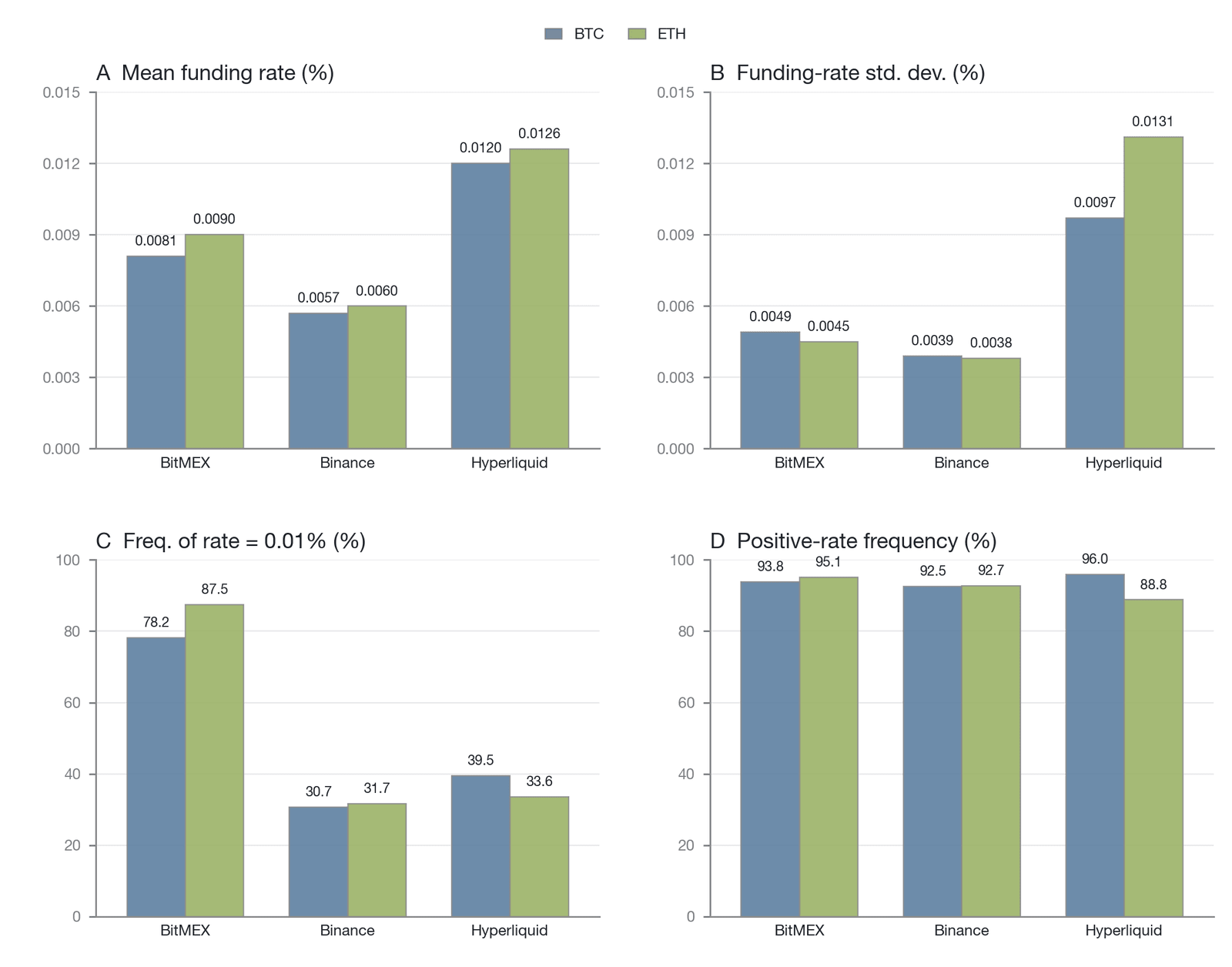
Figure 10-2. Comparison of the statistical characteristics of BTC and ETH funding rates on major exchanges in Q3 2025 [8]
As Figure 10-2 shows, the rate behavior of the three exchanges differs markedly. BitMEX's BTC rate was stable at 0.01% for 78.2% of the time (panel C), with a standard deviation of only 0.0049%, exhibiting high predictability. Binance, the world's largest exchange, had a mean rate (0.0057%) that was actually lower than BitMEX's (0.0081%), reflecting persistent short-side pressure on the Binance platform—possibly from the large numbers of hedge funds and market makers that establish short positions on Binance to hedge long exposure on other platforms. Hyperliquid's mean rate (0.0120%, panel A) and standard deviation (0.0097%, panel B) were both significantly higher than those of the two centralized exchanges, with a maximum of 0.0672%, exhibiting higher volatility and greater sensitivity to market sentiment [8].
| Exchange | BTC mean rate | BTC standard deviation | Frequency of BTC rate = 0.01% | Frequency of positive BTC rate |
|---|---|---|---|---|
| BitMEX | 0.0081% | 0.0049% | 78.19% | 93.83% |
| Binance | 0.0057% | 0.0039% | 30.70% | 92.54% |
| Hyperliquid | 0.0120% | 0.0097% | 39.45% | 95.98% |
Table 10-3. Core statistical indicators of BTC funding rates on three exchanges in Q3 2025 [8] (Data source: compiled by the author based on [8])
One shared feature stands out: despite the vast differences in design parameters and rate volatility across the three exchanges, the frequency of positive BTC rates exceeded 92% on all of them (Table 10-3). This means that throughout Q3 2025, on every platform, longs paid shorts more than 90% of the time. This phenomenon is not accidental but the joint result of the institutional benchmark set by the interest rate component I = 0.01% and the structural positive bias of the clamp function: even in periods when the market's directional preference is relatively neutral, the "default state" of the rate is positive. In its report, BitMEX calls this phenomenon the "formula's secret positive bias" [8].
These cross-exchange parameter differences and statistical patterns are not minor technical details. They determine the thickness and response speed of arbitrage capital on each platform, the cost and feasibility of a "rate squeeze" attack by a manipulator, and the speed and magnitude of rate polarization during extreme conditions. More importantly, they constitute the initial conditions for all the analysis that follows in this chapter: the "three-layer decomposition model" of Section 10.2 explains why these parameter differences produce institutional friction layers of differing sizes; the "anchoring strength spectrum" of Section 10.3 argues how different designs affect the effectiveness boundary of anchoring; the "three-layer game model" of Section 10.4 analyzes how parameter differences alter the equilibrium structure of each layer of the game; and Section 10.7 examines settlement frequency as a core design dimension.
10.2 The three-layer decomposition model
In the crypto derivatives market, traders often treat the funding rate simply as a "directional indicator of long-short forces" or a "market sentiment gauge." This one-dimensional understanding, however, obscures the microstructural complexity of the funding rate. To accurately parse the market signal the funding rate conveys, we must abandon the view of it as a single variable and instead adopt a three-layer decomposition model. The model deconstructs the observed surface funding rate into three decomposable components with distinct economic meanings: the financing cost layer, the sentiment premium layer, and the institutional friction layer. The institutional friction layer, however, is not statistically orthogonal to the sentiment premium layer P but mechanically dependent on it through the clamp function.
10.2.1 The financing cost layer
The bottom layer of the funding rate is the financing cost layer, which represents the capital cost implied by holding a derivatives position under a risk-free-arbitrage assumption. This layer makes the funding rate of perpetual futures not merely a tool for adjusting a relative price, but also an expression of an absolute rate of return.
Before analyzing each layer, consider the architecture of the three-layer decomposition model as a whole. Figure 10-3 arranges the three components of the rate from lowest to highest by their frequency of variation.
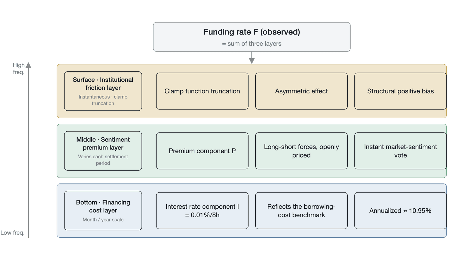
Figure 10-3. The three-layer decomposition model of the funding rate
As Figure 10-3 shows, the financing cost layer forms the base benchmark of the rate, maintaining a default state near 0.01% in the absence of extreme market deviation; the sentiment premium layer is superimposed on the financing cost layer and fluctuates in real time with shifts in long-short forces; and the institutional friction layer imposes a nonlinear truncation on the combined result of the first two layers through the clamp function, producing the structural positive bias of the rate distribution. The interaction of the three layers determines the actual observed rate at any moment.
In the funding rate formulas of most major crypto exchanges (such as BitMEX and Binance), the financing cost layer is hard-coded as a fixed interest rate component (usually denoted I). For example, BitMEX initially set the benchmark rate at 0.01% every 8 hours, equivalent to an annualized rate of about 10.95% (simple annualized, i.e., ; compounded, it is about 11.57%, i.e., ) [8]. This setting is not an arbitrary mathematical constant but an empirical estimate based on the difference in borrowing costs between the U.S. dollar (or stablecoins) and Bitcoin in the early crypto market. It constitutes a form of institutional rigidity: after the Federal Reserve raised its benchmark rate to 5.25% in 2023, the premium of the crypto market's fixed 10.95% interest rate component over the traditional risk-free rate was sharply compressed (from more than 10 percentage points in the zero-rate era to about 5.7 percentage points), yet the formula itself was not dynamically adjusted.
The borrowing cost hypothesis holds that a buyer of perpetual futures is effectively borrowing the quote currency (such as USDT) to purchase the underlying asset (such as BTC), while a seller is borrowing the underlying asset to obtain the quote currency. The benchmark of the funding rate should therefore reflect the interest rate spread between these two assets in the spot lending market. Because demand for stablecoin borrowing in the crypto market has long exceeded demand for borrowing native crypto assets, this structural supply-demand imbalance has made stablecoin lending rates significantly higher than crypto-asset lending rates, which is then embedded at the formula level as a persistently positive interest rate component.
10.2.2 The sentiment premium layer
Above the financing cost layer sits the highly dynamic sentiment premium layer, the part of the funding rate that traders watch most closely. The sentiment premium layer is composed of the premium component (usually denoted P), which measures in real time the deviation between the perpetual futures price and the spot index price. The sentiment premium layer is the direct result of the game between long and short forces in the market microstructure and represents the open-market pricing of risk. When the market expects prices to rise, speculative long forces strengthen and push up the perpetual price, so that P > 0; conversely, when the market expects a decline, short forces dominate, so that P < 0. During the bull phase of November 2024, when Bitcoin broke $100,000, the premium component of BTC perpetual futures stayed persistently in the elevated range of 0.05% to 0.15%, reflecting a concentrated influx of leveraged long demand; whereas during the AI-sector turbulence triggered by DeepSeek in late January 2025, the premium component of some altcoins plunged below −0.3%, revealing the impact of panic selling on the microstructure of the derivatives market.
In a normal market environment with sufficient arbitrage capital, the sentiment premium layer reflects the risk compensation that arbitrageurs demand for absorbing one-sided market imbalances. In their study of crypto carry, Schmeling et al. at the Bank for International Settlements note that the arbitrage returns of crypto futures are essentially a highly volatile "convenience yield," one arising from the trend-following behavior of retail investors chasing leveraged upside exposure and from the relative scarcity of arbitrage capital willing to bear basis risk [12]. The sentiment premium layer is therefore not merely a measure of sentiment but the pricing that market liquidity providers (arbitrageurs) place on the use of their capital.
10.2.3 The institutional friction layer
The component of the three-layer decomposition model that is often overlooked yet plays a significant role in actual operation is the institutional friction layer. This layer arises from the mathematical truncation mechanism—the clamp function—that exchanges deliberately introduce to prevent the funding rate from fluctuating excessively. BitMEX introduced this mechanism when it designed perpetual futures in 2016, with the aim of preventing extreme single-period rate fluctuations from triggering chain liquidations, while also providing arbitrageurs with a predictable return floor to sustain their participation. The final funding rate formula of most exchanges can be written as . This seemingly simple smoothing mechanism creates a significant asymmetric effect at the microstructural level.
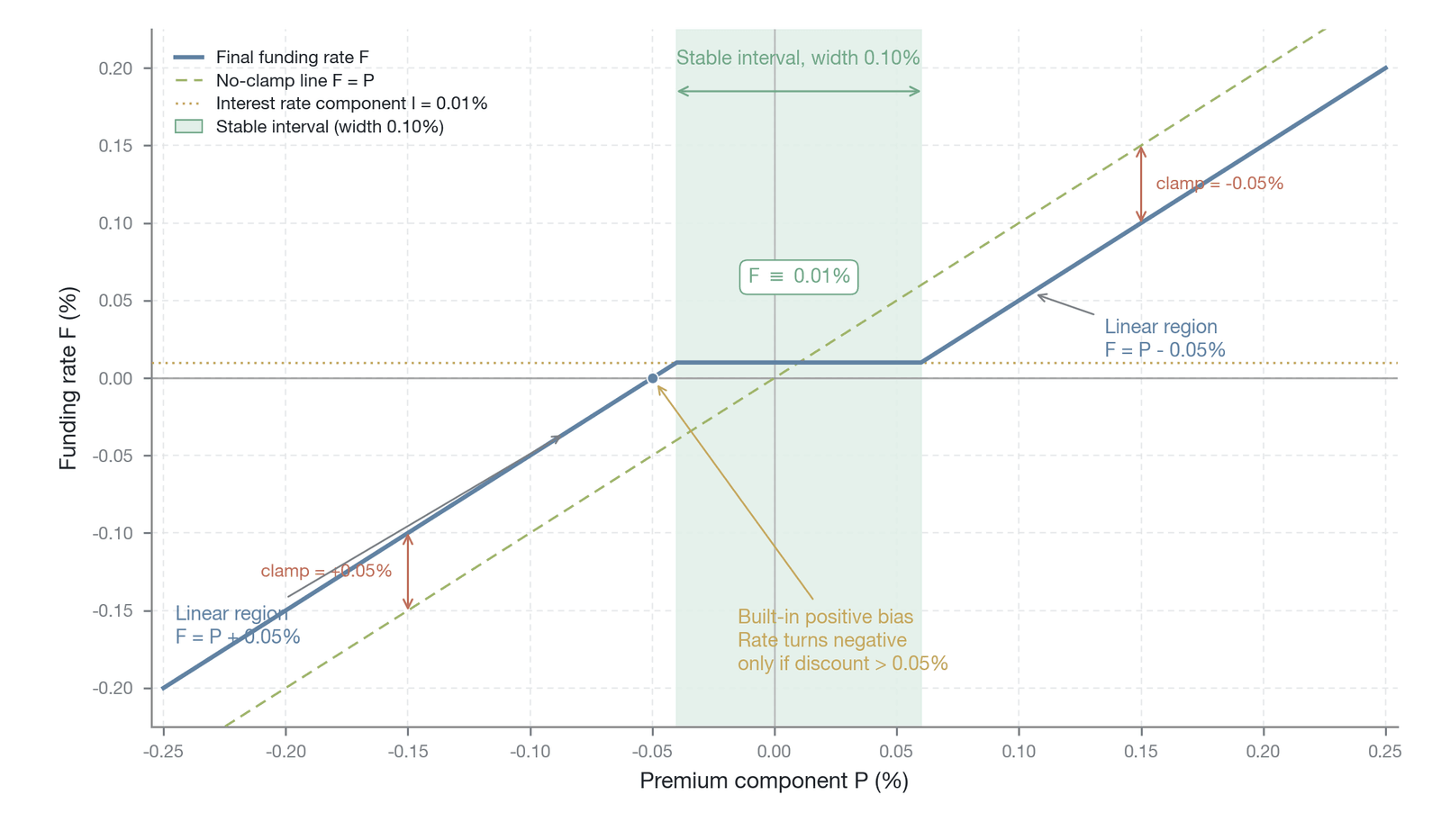
Figure 10-4. The asymmetric truncation effect of the clamp function on the funding rate and the resulting stable band (a conceptual illustration derived from the formula, not empirical data; the clamp thresholds of about ±0.05%, the interest rate component of 0.01%, and the stable-band width of 0.10% are all formula constants [8])
As Figure 10-4 shows, the clamp function creates a "stable band" 0.10% wide (when the premium component P lies between −0.04% and +0.06%). Within this band, the truncation term in the formula offsets fluctuations in the premium, forcing the final funding rate to be anchored at I = 0.01%.
This mechanism produces a structural positive bias in the funding rate distribution. Even when the perpetual futures are at a slight discount (for example, P = −0.03%), the intervention of the clamp function still requires longs to pay shorts a funding rate of 0.01%. Only when the discount exceeds −0.05% does the funding rate fall to zero; only when the discount is deeper still does the rate turn negative.
BitMEX's Q3 2025 derivatives report corroborates this structural feature (Figure 10-2): the BTC funding rate was exactly equal to 0.01% for as much as 78.19% of the time and remained positive 93.83% of the time [8], and even the more volatile Hyperliquid had a positive-rate share as high as 95.98%. This shows that the widespread "persistently positive rate" phenomenon in the market is largely not the result of sustained market optimism but of the institutional friction layer—that is, the formula's built-in positive bias.
10.2.4 Macro interest rate resonance and the economics of arbitrage
Having decomposed the funding rate, we can compare its financing cost layer with the macroeconomic environment to reveal the economic drivers of cross-market arbitrage. Figure 10-5 compares the divergence between the Federal Reserve's benchmark rate and the implied rate of perpetual futures from 2020 to 2025, along with the evolution of the resulting cross-market arbitrage spread.
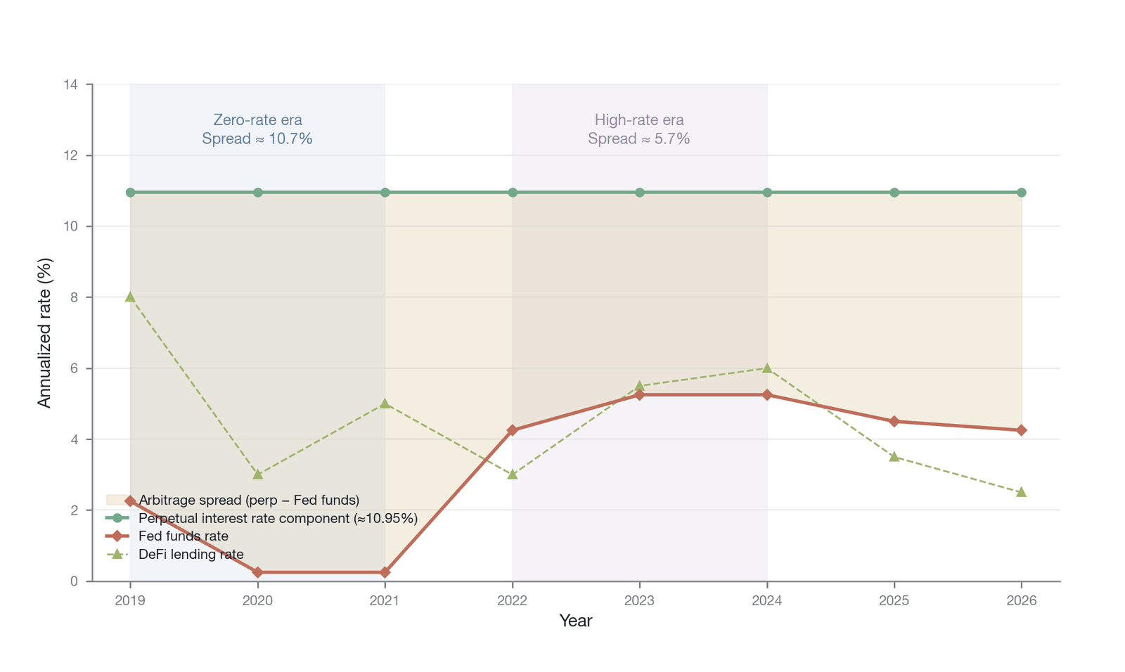
Figure 10-5. The divergence between the macro interest rate environment and the implied rate of perpetual futures, and the resulting arbitrage space (an illustrative trend chart, not a true month-by-month series; the Federal Reserve path is public macro data, the perpetual implied rate of about 10.95% annualized is an arithmetic formula constant, and the narrowing-spread trend is consistent with Bloomberg reporting [13])
As Figure 10-5 shows, the interest rate component of perpetual futures (about 10.95% annualized) was fixed at the outset. During the "zero-rate era" of 2020–2021, the Federal Reserve's benchmark rate was near zero and risk-free returns in traditional financial markets were extremely low. At that time, the crypto market's benchmark funding rate of more than 10% created a large cross-market arbitrage spread (exceeding 10%). This large spread attracted substantial traditional institutional capital (such as early crypto hedge funds) into the crypto market to execute cash-and-carry arbitrage, providing ample liquidity to the market.
Entering the "high-rate era" of 2023–2024, however, the Federal Reserve's benchmark rate climbed above 5.25% and traditional risk-free yields rose sharply. At this point, the advantage of the crypto market's fixed interest rate component over the traditional dollar risk-free rate was greatly compressed, and the arbitrage spread narrowed to around 5%. This change in the macro environment raised the marginal opportunity cost of arbitrage capital. As Bloomberg reported in early 2026, with basis yields falling to around 5%, Wall Street hedge funds began retreating from the Bitcoin basis trade [13].
Beyond the price signal of a narrowing spread, rising macro interest rates also weaken the anchoring strength of perpetual futures through two overlooked channels. The first is structural diversion through the ETF/CME channel: after the approval of BTC spot ETFs in January 2024, institutions could construct arbitrage using ETFs plus CME futures without bearing the counterparty risk of crypto-native exchanges. This is not merely a total retreat driven by a narrowing spread but a structural migration of arbitrage capital from crypto-native platforms to traditional financial infrastructure; institutions no longer need to bear exchange credit risk on Binance or Bybit to capture basis yield. The second is quantity contagion and risk-appetite contagion: rising macro interest rates weaken anchoring strength not only through the price signal (a narrowing spread) but also directly through quantity shocks (redemptions by liquidity providers, which force compliant funds to withdraw arbitrage positions) and risk-appetite contagion (a macro risk-off that drives down crypto prices and triggers a liquidation cascade). These three contagion channels—a narrowing spread, structural diversion of capital, and risk-appetite transmission—together explain why the arbitrage depth of the perpetual futures market has declined structurally since 2023.
This resonance and divergence of macro interest rates explains why the liquidity depth and the abundance of arbitrage capital in the crypto derivatives market differ significantly across macro cycles. Now that the Federal Reserve has begun its rate-cutting cycle in the second half of 2025, the decline in traditional risk-free yields will again widen the crypto market's arbitrage spread and may attract a return of the institutional capital that had previously retreated. Meanwhile, on-chain DeFi lending rates (such as the floating borrowing rate for USDC on Aave) provide a more real-time dynamic proxy for the financing cost layer, and the spread between them and the funding rate of perpetual futures constitutes a driver of cross-protocol arbitrage.
10.2.5 Empirical methods for separating the three layers
In empirical research and quantitative trading, accurately separating these three components is a prerequisite for constructing effective strategies. Quantitative researchers typically use the following methods to separate them (Table 10-4):
| Component | Observation and separation method | Economic meaning | Trading strategy application |
|---|---|---|---|
| Financing cost layer () | The exchange's publicly disclosed fixed parameter (usually 0.01%/8h), or a dynamic proxy estimate via a DeFi stablecoin lending rate (such as the Aave USDC borrowing rate). | The time value of capital and the cross-market risk-free interest rate benchmark. | Serves as the benchmark return for cross-market arbitrage and helps assess the opportunity cost of arbitrage capital. |
| Sentiment premium layer () | Computed from high-frequency order-book data as the real-time basis between the perpetual futures (traded price/mid-price) and the spot index price. | Pure market-microstructure imbalance and one-sided speculative momentum. | Building momentum or mean-reversion strategies; identifying extreme sentiment-reversal points. |
| Institutional friction layer | In the frictionless limit, (the premium cancels out), so the institutional friction term should be measured by the amount of truncation: , i.e., the extent to which the clamp truncates . | The intervention and distortion of the market's natural clearing process by exchange rules. | Finding structural mismatches where the market is "at a discount but the rate is still positive" and building statistical-arbitrage strategies with a positive expectation. |
Table 10-4. Empirical methods for separating the three components of the funding rate (Data source: compiled by the author)
The three-layer decomposition model is not the only framework for explaining the drivers of the funding rate. In the traditional finance literature, several competing theories exist for the pricing of the futures basis. The convenience yield hypothesis holds that holding the spot asset itself carries an implicit value (such as voting rights, staking rewards, or immediate availability), and this value should be reflected in a futures discount. In the crypto context, the convenience yield of holding spot BTC may include the opportunity cost of on-chain staking or DeFi participation. The hedging pressure hypothesis emphasizes that when producers (analogous to miners or token issuers in the crypto market) systematically short futures to lock in forward prices, the concentrated supply of shorts depresses the futures price and produces a negative basis unrelated to speculative demand. The market segmentation hypothesis notes that if participants in the spot and derivatives markets differ systematically in capital, information, or access, the prices of the two markets can diverge persistently without being arbitraged away. The three-layer decomposition model adopted in this chapter does not reject these theories but incorporates part of their insights into different layers: the effects of convenience yield and hedging pressure are absorbed by the sentiment premium layer, while market segmentation is reflected indirectly through the arbitrage-impediment conditions (Section 10.3.3). A rigorous empirical test, however (such as a regression that decomposes the rate into convenience-yield and speculative-sentiment components), is left to future research.
Through the three-layer decomposition model, we recognize that the funding rate is not a freely floating price determined purely by market supply and demand but a hybrid indicator deeply shaped by institutional rules. In interpreting the funding rate signal, a trader must strip away the "pseudo-steady state" caused by the institutional friction layer and the "positive bias" caused by the financing cost layer in order to reach the true market-microstructure state reflected in the sentiment premium layer.
10.3 The anchoring strength spectrum
In traditional futures markets, the physical or cash delivery mechanism at expiry provides a kind of "hard anchor." No matter how far a contract deviates from the spot price during its life, at the moment of expiry the futures price and the spot price must forcibly converge, or else a risk-free, deterministic arbitrage opportunity would arise. Perpetual futures, however, have no expiry date, and the convergence of their price toward the spot price depends entirely on the funding rate mechanism. This mechanism, which relies on continuous payments, is called a "soft anchor."
The key to understanding the perpetual futures market is to recognize that this soft anchoring is not a binary, black-or-white state (either anchored or unanchored) but a continuous anchoring strength spectrum.
10.3.1 Defining anchoring strength
We can introduce a parameter α (anchoring strength) between 0 and 1 to quantify this concept. Operationally, α can be estimated from the half-life of the deviation of the perpetual futures price from the spot price: the shorter the half-life, the faster the deviation is corrected and the higher the anchoring strength. When α = 1, anchoring is perfect, equivalent to the hard-delivery state of traditional futures at expiry, with the futures price F_t strictly equal to the spot price S_t. When α = 0, there is no anchoring, and the perpetual futures degenerate into a purely speculative instrument entirely unconstrained by the spot price, with its price determined solely by the internal long-short game of the derivatives market. In actual perpetual futures markets, anchoring strength always lies on a continuous spectrum with 0 < α < 1. Operationally, α can be estimated with an error correction model. Let be the basis at time t; the dynamics of the basis can be modeled as:
where κ > 0 is the mean-reversion speed parameter and is a white-noise disturbance. The larger κ is, the faster the basis is corrected and the tighter the anchoring. The operational proxy for α is , with a corresponding half-life of . In a normal market environment, based on high-frequency basis data from BitMEX and Binance, a preliminary estimate from an error correction model suggests that h is about 2 to 4 hours—that is, half of the basis is corrected by arbitrage activity within 2 to 4 hours (corresponding to a cumulative correction of about 75%–94% of the basis within 8 hours and about 94%–99.6% within 16 hours). During extreme events (such as Black Thursday in March 2020), however, h can exceed 48 hours (corresponding to α < 0.2), indicating that the anchoring mechanism has almost completely failed. The estimated value of κ depends heavily on data frequency, and during extreme events exhibits fat tails, which may bias the OLS estimate. A more refined Markov regime-switching model can capture the switching of κ across three states—normal, stress, and crisis—though its estimation and testing are left to future research. The half-life parameters above should be understood as preliminary estimates based on descriptive analysis in this book, not as rigorous econometric test results.
In the overwhelming majority of normal market periods, α is close to 1 (for example, α ≈ 0.9), and the funding rate effectively constrains the perpetual futures price to near the spot price.
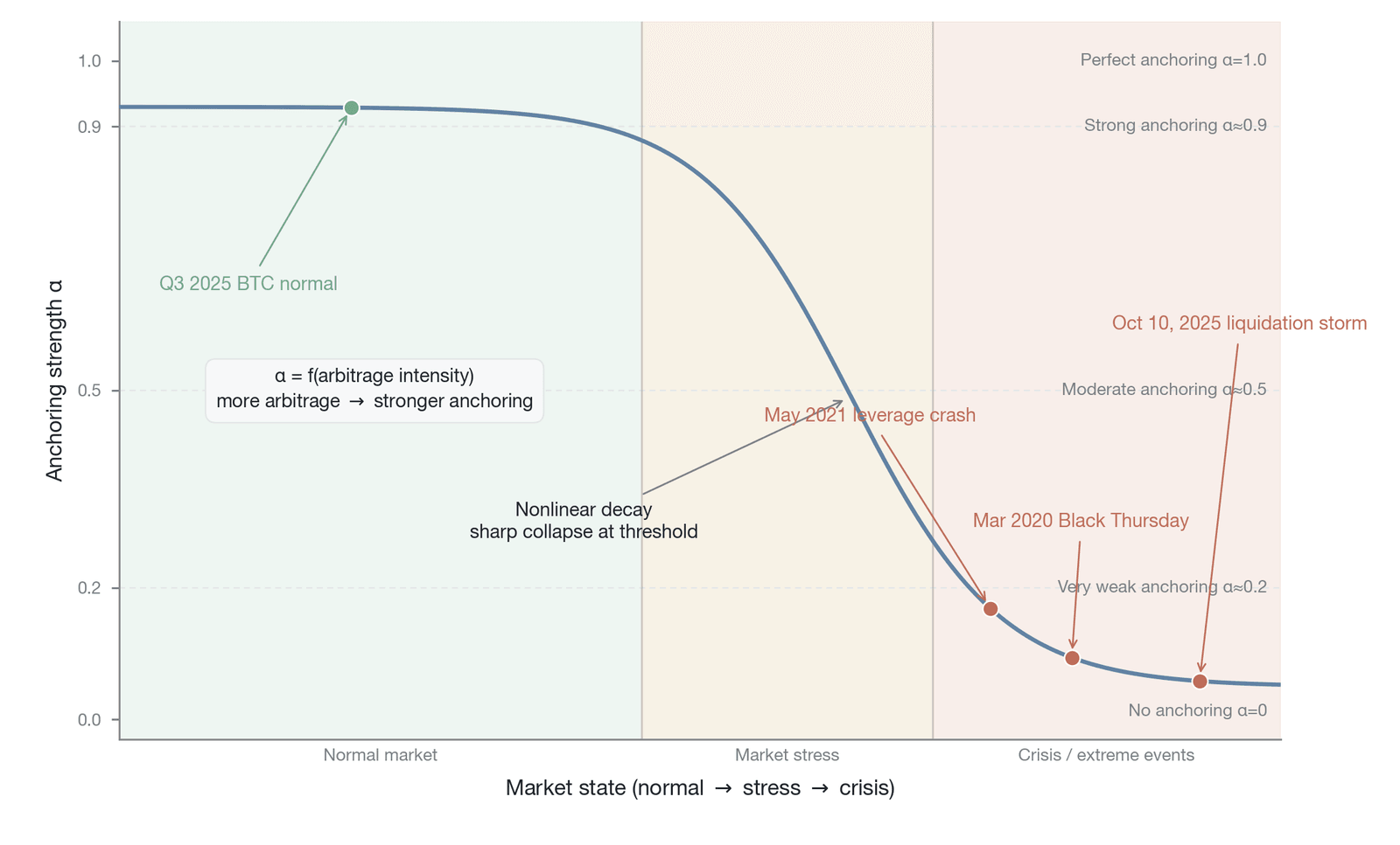
Figure 10-6. The anchoring strength spectrum and deviations during extreme events (a conceptual illustration, not empirical data; the anchoring strength α is a model parameter defined in this book and an author's estimate)
As Figure 10-6 shows, anchoring strength remains in the high range of 0.8 to 0.95 in a normal market environment, and the deviation between the perpetual futures price and the spot price is usually no more than 0.1%. When the market enters an extreme event (such as Black Thursday in March 2020 or the leverage crash of May 2021), anchoring strength plunges below 0.2, and the perpetual futures price deviates persistently from the spot price by hundreds of dollars. This nonlinear decay characteristic shows that the anchoring efficacy of the funding rate does not decline along a linear path but collapses abruptly at a particular threshold.
10.3.2 Arbitrage activity and anchoring strength
The funding rate formula is merely a calculation rule and has no direct power to pull prices. The formula does not create anchoring; it only creates the profit space for arbitrage. What truly creates anchoring is the arbitrage capital drawn in by that profit. When the perpetual futures are at a premium (P > 0), the funding rate is positive. Arbitrageurs construct a market-neutral portfolio by "shorting the perpetual + buying spot," thereby collecting the funding rate risk-free. This operation generates sell pressure in the derivatives market (depressing the contract price) and buy pressure in the spot market (raising the spot price), physically forcing the two prices to converge.
Ackerer, Hugonnier, and Jermann (2025) propose the AHJ framework [14] and prove this under the assumption of a frictionless, continuous-trading market. They show that the price of perpetual futures can be expressed as the risk-neutral expectation of the spot price sampled at random time points that reflect the strength of price anchoring. This anchoring strength, at the microstructural level, depends primarily on the smoothness of dynamic trading and the replication of primitive securities—that is, on the efficiency of arbitrage activity.
We can therefore draw a core conclusion: α is a monotonically increasing function of the intensity of arbitrage activity. This conclusion is highly consistent with the intermediary asset pricing theory of Gabaix and Maggiori (2015) [15]. In their framework, the degree of asset-price deviation depends not on changes in fundamentals but on the capital adequacy of financial intermediaries (in this context, arbitrageurs): when intermediary capital contracts, price deviations widen sharply even if fundamentals are unchanged. The anchoring strength of perpetual futures is precisely a direct mapping of this theory onto the crypto derivatives market: the capital condition of arbitrageurs determines the effectiveness boundary of the soft anchor. This can be formalized as , where A is the total amount of active arbitrage capital in the market, L is the liquidity depth for cross-market execution, and σ is the current volatility level. As long as arbitrage channels are unobstructed, capital is abundant, and volatility is within a controllable range, the funding rate can anchor prices effectively; but once A plummets because of capital retreat, L dries up because market makers pull their orders, or σ spikes above arbitrageurs' risk-control thresholds, anchoring strength slides rapidly toward 0.
10.3.3 Conditions that impede arbitrage
If arbitrage activity is the sole source of anchoring strength, then the question of "why the rate fails" becomes "why arbitrage is impeded." In extreme market turmoil, arbitrageurs often face the following six impediment conditions, which prevent them from executing the arbitrage that should flatten the basis and thereby trigger an anchoring collapse.
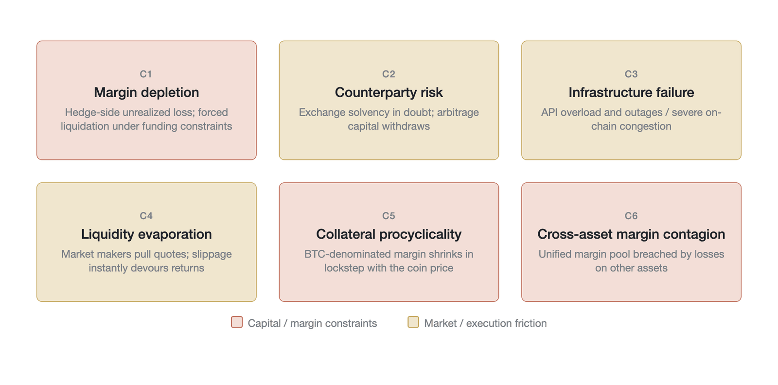
Figure 10-7. The six arbitrage-impediment conditions that cause the anchoring of perpetual futures to collapse
Margin depletion is the primary impediment. In a violent one-sided market, an arbitrageur's hedged position may face large paper losses. Although the overall portfolio is market-neutral, the paper losses on the derivatives leg require continuous margin top-ups. If an arbitrageur faces a liquidity constraint and cannot replenish fiat or stablecoin margin in time, it risks forced liquidation. This mechanism corresponds closely to the spiral between market liquidity and funding liquidity proposed by Brunnermeier and Pedersen (2009) [16]. In their theoretical framework, a decline in asset prices tightens traders' margin constraints, forcing them to cut positions; the position-cutting further depresses prices, forming a self-reinforcing deleveraging loop. Margin depletion among arbitrageurs in the crypto market is precisely the concrete manifestation of this funding-liquidity spiral in the perpetual futures market: arbitrageurs exit not because their strategy has failed but because their funding constraint has been breached. At the same time, counterparty risk intensifies. When systemic risk emerges, arbitrageurs worry about the solvency of the exchange itself. If they expect the exchange might go bankrupt or restrict withdrawals, arbitrage capital will choose to withdraw to protect principal no matter how high the funding rate, creating a vacuum of arbitrage force. In addition, infrastructure failures tend to erupt at critical moments. Arbitrage relies on high-frequency, low-latency cross-market operations, and in extreme conditions an exchange's API may become overloaded and go down, or the underlying blockchain network may become severely congested. Liquidity evaporation further worsens the arbitrage environment: as panic spreads, market makers cancel orders to avoid risk, leaving the order book extremely thin. At this point, arbitrageurs face enormous slippage costs when establishing or unwinding spot and derivatives positions, which can instantly wipe out months of funding-rate returns and make arbitrage economically infeasible. Collateral procyclicality further aggravates the situation: in the early, BTC-margined perpetual futures, when the BTC price crashed, short arbitrageurs faced not only the pressure of a falling contract price but also a simultaneous shrinkage in the fiat value of the BTC they used as margin. This double effect significantly amplified liquidation risk, forcing arbitrageurs to close positions passively at the very moment the market most needed liquidity.
Beyond these five conditions, cross-asset margin contagion constitutes a sixth, often-overlooked arbitrage-impediment condition. Under the unified margin mode of exchanges such as Binance and Bybit, an arbitrageur's BTC cash-and-carry position may share a margin pool with positions in other assets. When another asset (such as LUNA in 2022) collapses, losses on that asset erode the unified margin, forcing the arbitrageur to close out an otherwise healthy BTC arbitrage position. This contagion path means that the anchoring strength of BTC can fall unexpectedly during a non-BTC event: arbitrageurs exit not because of pressure in the BTC market itself but because they are breached by risk spillover from other assets. During the LUNA/UST collapse of May 2022, some arbitrage funds operating under the unified margin mode were forced to liquidate their market-neutral positions in both BTC and ETH simultaneously, providing empirical support for this contagion path.
10.3.4 The AHJ framework: applications and limitations
The AHJ framework lays a solid mathematical foundation for the no-arbitrage pricing of perpetual futures in theory, proving that under the assumption of a perfect (frictionless, continuous-trading) market, a specific funding rate setting makes the perpetual futures price converge to the spot price [14].
When this theoretical framework is applied to the real crypto market, however, its limitations become fully apparent. The core assumptions of the AHJ model are a frictionless market and continuous trading capability. As the arbitrage-impediment conditions analyzed above show, the crypto market exhibits precisely the opposite at extreme moments: extremely high friction (slippage, congestion) and discontinuity of trading (outages, circuit breakers).
The AHJ framework therefore depicts the ideal state of α ≈ 1 in Figure 10-6. It explains why the funding rate can operate effectively during the 99% of the time that is normal, but it cannot explain why a deep price dislocation arises during the 1% "crisis moments." The no-arbitrage condition exhibits significant fragility when confronting a systemic liquidity shock.
10.3.5 The anchoring paradox
Taken together, these observations point to a core microstructural paradox of the crypto derivatives market: the anchoring paradox. When the market is calm and volatility is low, the natural deviation between the perpetual futures price and the spot price is already small. At such times, arbitrage channels are unobstructed, liquidity is ample, the funding rate mechanism operates effectively, and anchoring strength is extremely high. Yet at such times the market does not truly "need" a powerful anchoring mechanism, because prices themselves have no impetus to derail.
Conversely, when the market suffers a black swan event, volatility spikes, and derivatives prices deviate sharply from spot prices out of panic or greed, this is precisely the moment when the market most needs the funding rate to anchor. But it is exactly at this moment that, because the six arbitrage-impediment conditions are triggered simultaneously, arbitrage capital retreats on a large scale or is even forcibly liquidated, causing the transmission mechanism of the funding rate to break down entirely and anchoring strength to fall to its lowest level.
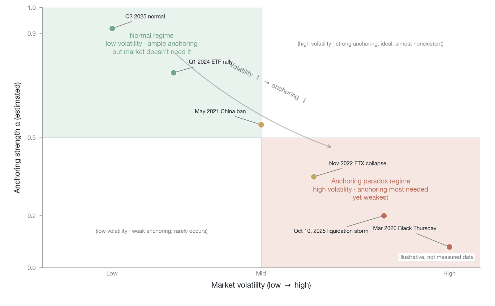
Figure 10-8. The inverse relationship between market volatility and anchoring strength (a conceptual illustration, not empirical data; the anchoring strength α is an estimate, the volatility axis is a qualitative scale of low, medium, and high, and the event points are qualitatively positioned)
As Figure 10-8 shows, the historical extreme events of the crypto market fully validate this paradox.
During the Black Thursday crash of March 12, 2020, the price of Bitcoin was cut in half in a single day. A post-mortem report by Multicoin Capital notes that, because of extreme congestion on the blockchain network and evaporated liquidity on BitMEX, arbitrageurs could not deposit BTC into BitMEX to flatten the spread [5]. Only about $20 million in bids remained on the entire BitMEX order book, yet it faced more than $200 million in long liquidations. The funding rate mechanism failed completely, causing the perpetual futures price on BitMEX to fall hundreds of dollars below other spot exchanges at one point (a discount of more than $500 at its peak, as noted in the chapter introduction) and nearly flash-crashing to zero.
Similarly, during the $19 billion liquidation storm of October 10, 2025, geopolitically induced panic caused liquidity across the entire market to evaporate instantly. Arbitrage capital was powerless in the face of extreme slippage and high network gas fees, causing the anchoring function of the funding rate to fail briefly and the basis to widen substantially [17].
The anchoring paradox reveals an inherent flaw of the funding rate as a "soft anchor": its effectiveness depends on market liquidity, yet it cannot itself create liquidity when liquidity dries up. This paradox is, in essence, a precise mapping of the "limits of arbitrage" theory of Shleifer and Vishny (1997) onto the crypto derivatives market [18]. Shleifer and Vishny note that real-world arbitrageurs are not the unconstrained agents of textbooks; they rely on external capital, and capital providers tend to withdraw funds precisely when arbitrage is most needed, because paper losses are most severe at that time. The anchoring paradox of perpetual futures is exactly the crypto version of this logic: arbitrageurs easily earn rate income when the market is calm but cannot perform their price-correction function under extreme deviations because of capital constraints and execution friction. This is the fundamental game-theoretic reason why the funding rate "works most of the time but occasionally fails at the most critical moment."
Several mechanism-design paths might alleviate the anchoring paradox, though each introduces new trade-offs. At least three are worth discussing. The first is the insurance fund as arbitrageur of last resort: the exchange actively executes cash-and-carry arbitrage during extreme basis events (as Hyperliquid's HLP vault plays a similar role in normal markets), but this turns the exchange from a neutral rule-setter into a direct market participant, introducing new conflicts of interest, and the size of the insurance fund may be far too small to fill the arbitrage vacuum in a systemic crisis. The second is an extreme-basis circuit breaker: pausing the liquidation engine when the basis exceeds a threshold, but pausing liquidations may cause greater risk accumulation (the paper losses of unliquidated positions keep expanding), and an intervention requiring human judgment is difficult to implement in a decentralized protocol. The third is dynamic rate-cap increases: automatically raising the rate cap in extreme states to strengthen negative feedback. But as the ALPACA case in Section 10.6.3 shows, an extreme rate can itself become a manipulation tool rather than a corrective force. Fully resolving the anchoring paradox may require introducing additional stabilization mechanisms beyond the rate mechanism, which constitutes an open research frontier in derivatives mechanism design.
10.4 The three-layer game model
The funding rate is not merely the result of a mathematical calculation but the product of a continuous game among multiple participants within a specific rule framework. To understand deeply how this mechanism operates in the crypto derivatives market, we construct a "three-layer game model." The model systematically deconstructs the formation and fragility of the funding rate's dynamic equilibrium at three levels: the microstructural confrontation of positions, the meso-level of cross-market arbitrage, and the macro-level of rule attack and defense.
10.4.1 The anchoring game
At the most microstructural level, the funding rate is essentially a near-zero-sum "war of attrition" between the long and short camps. When the perpetual futures price exceeds the spot index price, the funding rate is positive and longs must pay shorts periodically; the reverse holds otherwise. This mechanism is designed to force prices back to their spot anchor by raising the holding cost in the direction of the deviation.
Figure 10-9 arranges the three games in a concentric-circle structure by participant scope and time scale.
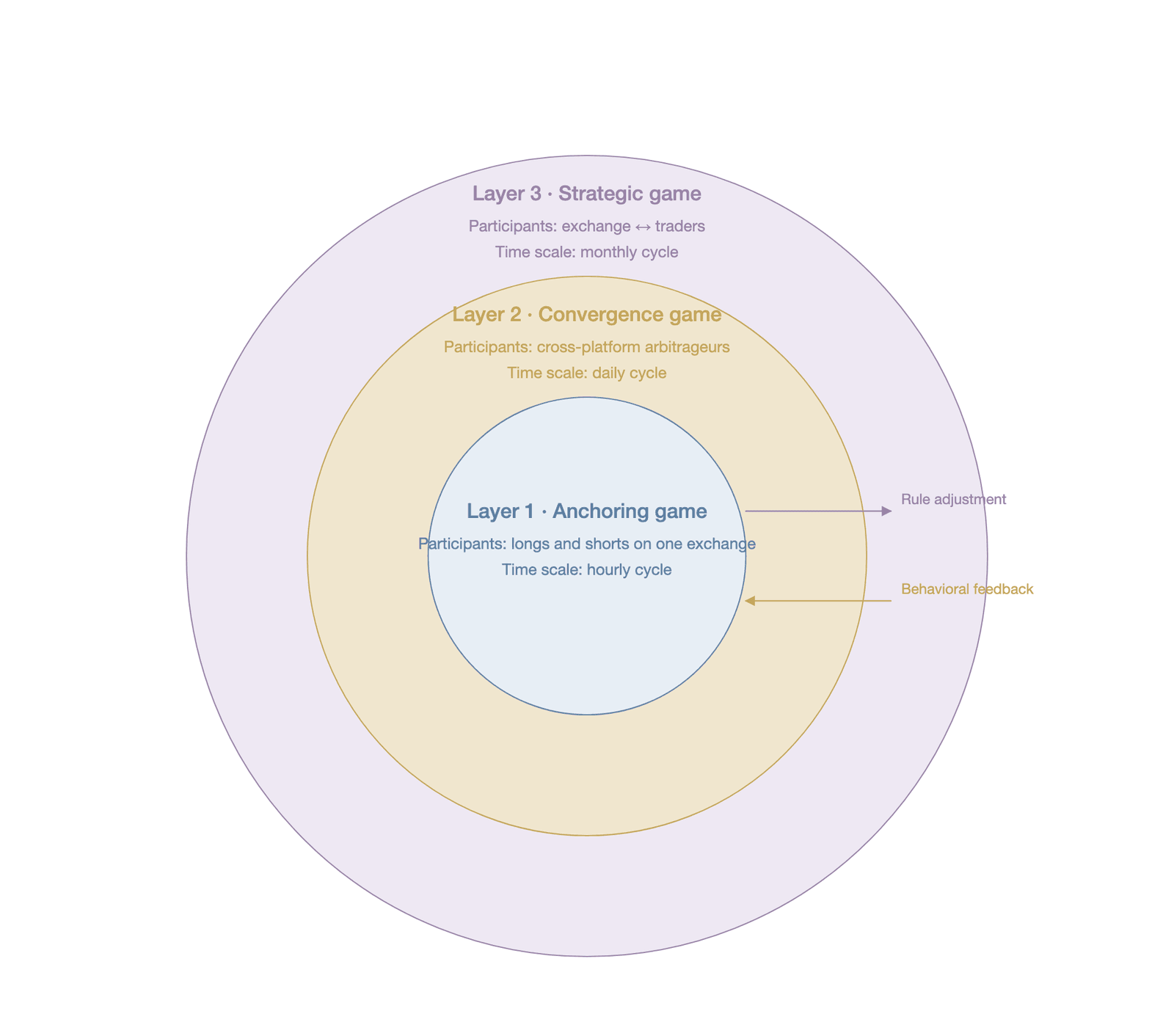
Figure 10-9. The nested structure of the three-layer game model of the funding rate
As Figure 10-9 shows, the three games exhibit a nested structure from the inside out: the innermost anchoring game determines the balance of long-short forces and the direction of the basis within a single exchange; the middle convergence game pulls prices and rates across platforms toward consistency through cross-market arbitrage; and the outermost strategic game determines the evolutionary path of the rules themselves. Feedback runs bottom-up among the three layers: imbalance in an inner game propagates outward, while rule adjustments in an outer layer alter the game structure of the inner layers.
To characterize the equilibrium structure of the anchoring game precisely, we model it as a 2×2 normal-form game. Consider a simplified single-period game in which longs and shorts each choose to "hold" or "exit." Let F be the current funding rate (paid by longs to shorts when positive), Δ the directional payoff expectation (positive favors longs), and λ the liquidation-risk loss triggered by a counterparty's exit. The payoff matrix is shown in Table 10-5:
| Short: hold (H) | Short: exit (E) | |
|---|---|---|
| Long: hold (H) | ||
| Long: exit (E) |
Table 10-5. The 2×2 normal-form payoff matrix of the anchoring game (Data source: compiled by the author)
The Nash equilibrium of this game depends on the size of the rate F relative to the directional payoff Δ and the liquidation risk λ. When (i.e., ), longs and shorts are mutual best responses, and (hold, hold) constitutes the unique pure-strategy Nash equilibrium (the upper bound is the short's tolerance condition and is the economically more binding side); both sides have an economic incentive to maintain their positions, and the anchoring game is in a steady state. When the rate rises to F > Δ + λ, the long's best response to the short holding becomes to exit (because ), while the short's best response to the long exiting is to hold (because ); the two are mutual best responses, and the equilibrium jumps to (exit, hold), which is precisely the condition under which the funding rate's negative feedback mechanism takes effect. When the directional payoff expectation becomes extreme (Δ ≫ F), however, the long's incentive to hold becomes unshakable, and even a persistently rising rate cannot trigger an equilibrium jump. In this state, the game slides from the "both hold" steady state into a positive-feedback regime, and the funding rate loses its corrective function. The analysis above assumes a single-period static game; in a multi-period dynamic game, reputation effects, learning, and strategic adaptation would further enrich the equilibrium structure, though its core dependence on the rate threshold would remain unchanged.
The analysis above also treats the directional payoff expectation Δ as an exogenous, commonly known parameter, but in practice longs and shorts hold systematically biased estimates of it. The heterogeneous-beliefs model of Scheinkman and Xiong (2003) [19] shows that overconfident longs systematically overestimate Δ, while shorts in a panic systematically underestimate it. More importantly, Δ is itself endogenous to the game: longs adding leverage and driving up the price raises the realized value of Δ ex post, forming a self-fulfilling prophecy. Treating Δ as an exogenous parameter obscures this reflexivity: longs and shorts do not face the same Δ but different values and weighted by their respective subjective probabilities, and these subjective beliefs are partly self-validating through their effect on the market price. This methodological qualification does not affect the qualitative conclusions of the equilibrium analysis above, but it indicates that a complete theoretical treatment requires a dynamic game framework with heterogeneous beliefs.
In actual operation, however, this war of attrition often exhibits strong reflexivity [20]. The noise-trader-risk model of De Long, Shleifer, Summers, and Waldmann (1990) provides a theoretical basis for understanding this phenomenon [21]. In their framework, even when rational arbitrageurs know that a price has deviated from fundamentals, the irrational behavior of noise traders may push the deviation further in the short run, exposing arbitrageurs to the risk of "being liquidated while on the right side." In the perpetual futures market, this noise-trader risk is sharply amplified by high leverage: arbitrageurs must bear not only the risk that the price deviates further but also the cash-flow pressure of the rate each settlement period, which can lead rational arbitrageurs to stay out even when the rate is extreme. In a bull cycle, longs expect the asset's price appreciation to far exceed the funding-rate cost they pay. Thus, even facing high holding costs, longs not only refuse to close positions but may use paper profits to add further leverage. This behavior widens the contract premium further, which in turn pushes the funding rate higher. At this point, the high funding rate is no longer a resistance that suppresses speculation but instead becomes a "confirmation signal" of the market's extreme optimism, attracting more speculative capital and forming a self-reinforcing loop of "rising price → rising rate → reinforced expectations → further position-adding."
The outcome of this war of attrition depends on the limits of each side's tolerance for cost. Although shorts can continuously collect risk-free rate income, they must bear the liquidation risk from further price increases. When market sentiment is extremely euphoric, the short camp may be forced to close positions because it cannot withstand the pressure of margin calls; this not only causes the price to spike instantly but also leaves the funding rate without a "counterparty" in the short term, further distorting the anchoring mechanism.
10.4.2 The convergence game
Without the intervention of an external force, the long-short war of attrition of the first layer easily falls into extreme imbalance. The core participants of the second-layer game are funding rate arbitrageurs, who, through cross-market operations, objectively bring about a dual equilibrium—price convergence and rate convergence—while pursuing risk-free returns.
Price convergence is achieved mainly through "cash-and-carry arbitrage." When the perpetual premium is too high (a positive funding rate), an arbitrageur buys the asset in the spot market while shorting an equal-size position in the perpetual futures market. This operation not only locks in the risk of price fluctuations but also steadily earns the funding rate. The arbitrageur's short-selling directly adds short-side force to the contract market, depressing the contract price and pushing it back toward the spot price.
Rate convergence is achieved through "cross-exchange arbitrage." Because different exchanges differ in liquidity depth, user composition, and rate-calculation details, the funding rate for the same asset often differs across platforms. Arbitrageurs short on the exchange with the higher rate and go long on the exchange with the lower rate, earning the rate spread between them. This capital flow ultimately flattens the rate differences across platforms. This convergence is limited, however, by the friction of transferring funds across platforms: transfers between CEXs involve withdrawal fees, on-chain confirmation delays (BTC takes 30–60 minutes), and anti-money laundering (AML) screening; transfers between CEXs and DEXs additionally involve the smart-contract risk of cross-chain bridging. These frictions determine the existence of a "no-arbitrage band": rate differences within the cost of cross-platform transfer cannot be eliminated by arbitrage, constituting the equilibrium width of the rate difference rather than a transient state converging to zero. According to Boros Finance's 2025 empirical research, cross-exchange rate arbitrage in BTC and ETH between Hyperliquid and Binance can achieve weighted-average fixed annualized returns of 5.98% to 11.4%, with peak returns in certain extreme periods exceeding 23% [22]. Because Boros is a provider of funding rate swap products, it reports gross returns before execution costs; actual net returns must deduct cross-exchange fund-transfer costs, the capital-efficiency loss from locking margin on two exchanges, slippage, and position-rebalancing friction, and may be significantly lower than the nominal figures.
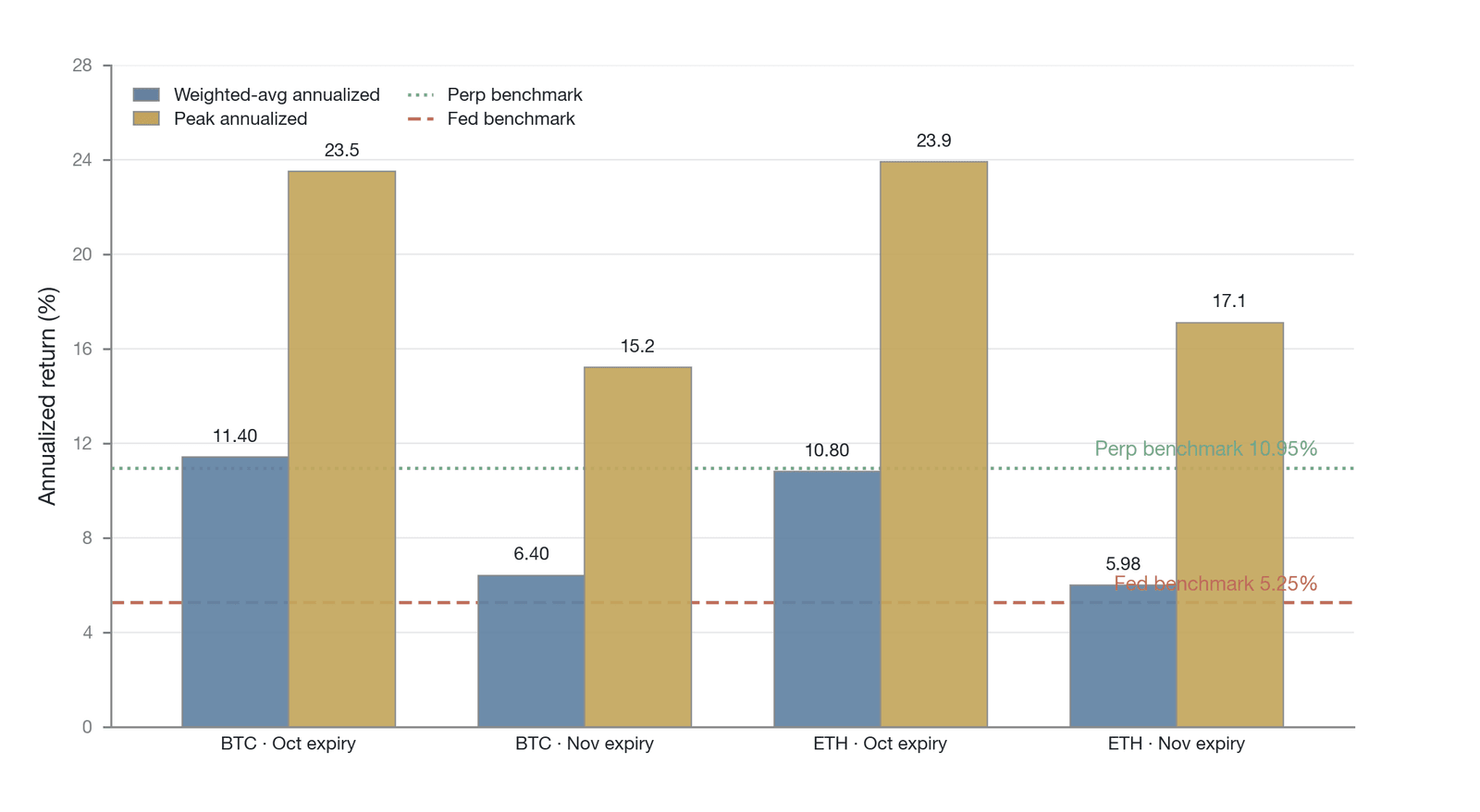
Figure 10-10. Annualized returns of cross-exchange funding rate arbitrage for BTC and ETH (gross returns before execution costs; BTC and ETH correspond to different maturities and are not a single-asset constant) [22]
As Figure 10-10 shows, the cross-exchange rate arbitrage returns for BTC and ETH exhibit pronounced time variation. The weighted-average annualized return for BTC was 11.4% (for the October 31 maturity) and 5.98% for ETH (for the November 28 maturity); note that the two correspond to different maturities and are not a single-asset constant, and the report shows gross returns before execution costs. Returns peaked in certain periods (exceeding 23%), typically corresponding to a widening cross-platform rate spread driven by extreme market sentiment. These high-return windows provide an economic incentive for arbitrage capital to enter, objectively promoting cross-platform convergence of the rate.
10.4.3 The strategic game
The third-layer game takes place between the rule-setters (exchanges) and the rule-adapters (traders). The exchange's goals are to maintain stable anchoring of the contract price, guard against systemic risk, and maximize trading volume; the trader's goal is to find loopholes within the rule framework to maximize profit.
To prevent excessive funding-rate fluctuations from causing large-scale chain liquidations, major exchanges generally set a rate clamp function and rate caps/floors. For example, BitMEX's empirical data show that under its clamp mechanism, the funding rate was fixed at the default 0.01% (every 8 hours) for as much as 78.19% of the time, equivalent to a benchmark annualized rate of about 10.95% [8]. Although such rules reduce day-to-day fluctuations, they also create space for rule arbitrage.
As the market has matured, this strategic game has intensified. For example, when some exchanges raised the settlement frequency from every 8 hours to every 1 hour or even real-time settlement, high-frequency traders quickly developed a "second-scale front-running" strategy, entering positions momentarily before settlement and exiting immediately afterward to capture rate income at no cost. As a countermeasure, exchanges (such as Binance in its September 2025 algorithm update) introduced a frequency normalization factor to eliminate this time-arbitrage space by smoothing the calculation window. This dynamic game of "rule-loophole discovery → strategy exploitation → rule patching" constitutes the underlying driver of the funding rate mechanism's evolution.
10.4.4 State dependence and the decay of anchoring efficacy
The validity of this three-layer game model is not fixed but highly dependent on the current market state. As the market moves from calm to extreme, the anchoring efficacy of the funding rate exhibits a pronounced nonlinear decay (Table 10-6).
| Market state | Basis characteristics | Core dominant force | Assessment of anchoring efficacy | Representative historical case |
|---|---|---|---|---|
| Normal state | Very small (< ±0.1%) | Rate arbitrageurs, market makers | Strong: arbitrage capital is ample, small deviations are quickly flattened, and the funding rate stays near its default benchmark. | Most of the calm trading periods in 2024–2025 |
| Stress state | Significant (±0.1% to ±1%) | Speculators (one-sided sentiment) vs. arbitrageurs | Weakened: one-sided sentiment widens the arbitrage space, but the execution constraints on arbitrage capital begin to appear, and the rate shows sustained positive or negative polarization. | The August 2024 yen carry-trade unwind shock; the AI-sector turbulence triggered by DeepSeek in late January 2025 |
| Crisis state | Extreme (> ±1%) | Liquidation mechanism (forced liquidation) | Failed: arbitrage channels break down entirely because of liquidity drought or network congestion, the liquidation mechanism takes over the market, and the rate mechanism no longer anchors but may instead accelerate the collapse. | Black Thursday on March 12, 2020; the leverage crash of May 19, 2021 [23] |
Table 10-6. State-dependent decay of the funding rate's anchoring efficacy (Data source: compiled by the author)
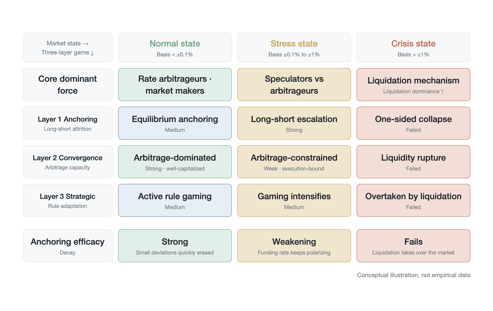
Figure 10-11. The relative strength of the three layers of game forces and the decay of anchoring efficacy across market states (a conceptual illustration, not empirical data; the strength of each layer is a qualitative rating of strong, medium, weak, or failed, and the basis thresholds are drawn from Section 10.4.4)
In the normal state, the second-layer convergence game (arbitrageurs) dominates, and the funding rate effectively anchors. When the market enters a crisis state, however (such as the May 19, 2021 crash in which the crypto market plunged 30% and more than $8 billion was liquidated market-wide [23]), arbitrageurs cannot execute cross-market operations because of spot-liquidity drought and severe network congestion. At this point, the second-layer game fails entirely, the first-layer long-short war of attrition devolves into one-sided chain forced liquidations, and the funding rate not only fails to pull prices back but its extreme negative values instead become a gauge of market panic.
In the crisis state, when the funding rate's anchoring mechanism fails and the liquidation cascade unfolds fully, the exchange's insurance fund and auto-deleveraging mechanism become the last line of defense for maintaining market continuity. The core function of the insurance fund is to absorb shortfall losses: when a position's liquidation price is worse than its bankruptcy price, the difference is borne by the insurance fund, thereby avoiding passing the shortfall on to the winning side. During Black Thursday on March 12, 2020, BitMEX's insurance fund drew down by about $8 million to $13 million (roughly 1,600 to 2,600 BTC) within a few hours, yet this was still insufficient to cover all shortfall losses [5]. When the insurance fund is exhausted, the auto-deleveraging (ADL) mechanism is triggered: the system automatically reduces counterparty positions according to a specific ranking algorithm to make up the shortfall. The ADL ranking algorithms of different exchanges differ significantly: BitMEX and Binance use a two-factor ranking of profit percentage and effective leverage, whereas Hyperliquid first uses HLP vault funds to absorb shortfall losses and triggers ADL against traders only when the HLP is insufficient. Systematic public data on the historical trigger frequency of ADL are currently lacking (flagged as an empirical-data gap), but Hyperliquid's on-chain transparency provides a data foundation for future empirical research.
The ADL mechanism fundamentally changes the payoff function of the game. In an ideal world without ADL, a trader's return is a deterministic function of directional judgment and leverage choice. But the existence of ADL means that even a trader who is right about direction and maintains prudent leverage may have profitable positions forcibly reduced during a liquidation cascade. The shortfall losses of a "neighbor who is right about direction but over-leveraged" are transmitted to the winning side through ADL. This creates a unique negative externality: the risk-taking of high-leverage speculators threatens not only their own survival but also, through the ADL mechanism, the return certainty of prudent traders. For the equilibrium of the anchoring game, the existence of ADL weakens arbitrageurs' incentive to participate: although arbitrageurs construct market-neutral portfolios, their profit leg still faces the tail risk of being forcibly reduced by ADL. This mechanism-design tension—the conflict between protecting system continuity and incentivizing arbitrage participation—remains an unresolved open problem in the mechanism design of perpetual futures.
Moreover, under a unified margin system, the rate polarization of one asset affects not only the game equilibrium of that asset itself but may also be transmitted to other assets through a shared margin pool. For example, when extreme negative rates on SOL cause SOL shorts to be liquidated, if those shorts hold ETH longs in the same margin pool, the ETH longs may also be liquidated by association, even if the ETH market itself shows no anomaly. This cross-asset contagion mechanism is developed further in the liquidation-cascade analysis of Chapter 11.
10.4.5 The structural boundaries of arbitrageurs
If arbitrageurs are the core force sustaining the funding rate's anchoring mechanism, why do they collectively "disappear" during extreme conditions? This stems from three structural boundaries that arbitrageurs face. As Figure 10-12 shows, all three constraints are loose in a normal market and arbitrage activity is unimpeded; when the market enters an extreme state, all three constraints tighten simultaneously and arbitrage capacity shrinks sharply.
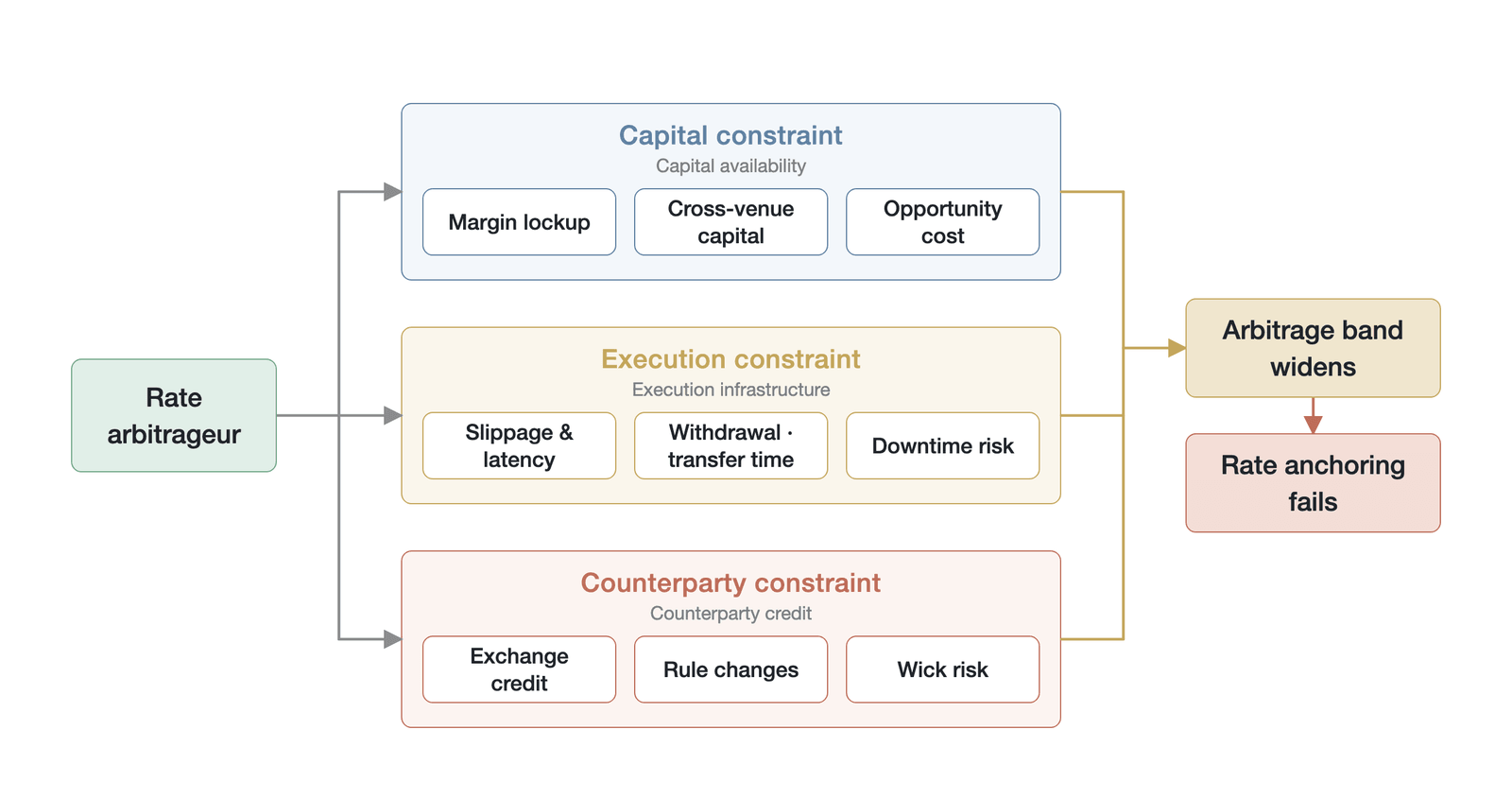
Figure 10-12. The three structural constraints faced by funding rate arbitrageurs
Gromb and Vayanos (2002) rigorously prove, from a general-equilibrium perspective, the systemic impact of capital constraints on arbitrageur behavior [24]. In their model, when arbitrageurs face funding constraints, the degree to which market equilibrium deviates from no-arbitrage pricing depends on arbitrageurs' wealth level: the poorer the arbitrageurs, the larger the price deviation and the more severe the welfare loss. This conclusion applies directly to the perpetual futures market: the persistent deviation of the funding rate (i.e., the decline in anchoring strength) essentially reflects the inadequacy of arbitrage capital relative to speculative demand.
These three constraints correspond mechanistically to the six arbitrage-impediment conditions of Section 10.3.3; rather than restate each one's operational details, we note only the core of each constraint. The capital constraint stems from the capital-intensity of cash-and-carry and cross-exchange arbitrage: arbitrageurs must reserve large redundant margins across multiple platforms to guard against one-sided liquidation, so capital efficiency is significantly reduced, and when the arbitrage space widens while idle capital runs out, the rate deviation persists. The execution constraint manifests as rate-limiting, latency, or even outages of exchange APIs during extreme conditions (such as the service disruptions at some leading exchanges on May 19, 2021 [25]), as well as delayed fund transfers caused by on-chain congestion and spiking gas fees. The counterparty constraint is the arbitrageur's passive exposure to the credit risk of centralized exchanges and to unilateral rule changes (such as forcibly rolling back trades, adjusting rate caps, or suspending withdrawals). These tail risks lead rational arbitrageurs to withdraw and wait on the sidelines precisely when the market most needs liquidity supply.
Together, these three constraints determine the capacity ceiling of the funding rate's anchoring mechanism. In quantitative terms, this ceiling depends on the total capital arbitrageurs can deploy, the speed of cross-platform fund transfers, and the credit rating of exchanges. In the BTC perpetual futures market, thanks to the participation of systematic arbitrage entities such as Ethena, arbitrage capacity is usually ample, whereas in the long-tail altcoin market, arbitrage capacity may be only a few million dollars, and a single medium-sized directional trade can breach this ceiling. When the corrective demand generated by a market deviation exceeds arbitrageurs' structural capacity, the equilibrium of the three-layer game model tends to collapse.
10.5 Rate polarization and positive feedback
In classical financial theory, the funding rate is designed as a negative feedback system: when the contract price deviates from spot, a rising rate increases the holding cost on the deviating side, forcing it to close positions or attracting arbitrageurs to enter, ultimately returning the price to spot and pulling the rate back down. In the extreme conditions of the crypto market, however, this negative feedback mechanism can flip and evolve into a self-reinforcing positive feedback system, driving the rate into extreme polarization.
10.5.1 Trigger conditions for positive feedback
The mathematical trigger condition for the flip from negative to positive feedback can be formalized as the following proposition.
Proposition (necessary condition for continued position-holding). Let be a trader's conditional expectation at time t of the next-period price change, F_t the current funding rate, γ the trader's risk-aversion coefficient, and t[\Delta P{t+1}] the conditional variance of the price change. When the following condition holds, a rational trader chooses to maintain the position and the funding rate's negative feedback mechanism fails:
t[\Delta P{t+1}]
The left side of this inequality is the expected return of holding the position, and the right side is the total cost of holding, comprising the deterministic rate outlay F_t and the risk-aversion-adjusted directional risk premium t[\Delta P{t+1}]. In the simplified version (setting γ = 0, i.e., the risk-neutral assumption), the condition reduces to —that is, the expected directional profit merely needs to exceed the rate cost. The full version introduces the risk-aversion coefficient, meaning that even if the expected return exceeds the rate, a risk-averse trader may still choose to exit if the directional risk is too large (high ). When the market narrative is highly certain (such as the ALPACA delisting announcement), traders tend to establish positions immediately, and positive feedback is more easily triggered. This analysis requires a finer distinction, however: a delisting announcement provides directional certainty (the price should fall) but increases uncertainty in magnitude and time path, and the price path before delisting may exhibit violent fluctuations and a short squeeze (as events indeed proved). The "focusing illusion" of behavioral finance (Kahneman 2011 [26]) may better explain this phenomenon: traders focus excessively on the directional narrative ("delisting = crash") while underestimating path risk, causing them to systematically overestimate the net expected return of establishing a position immediately.
The inequality above characterizes only the static decision condition under which a holder does not exit; it is necessary but not sufficient for positive feedback to form. Positive feedback also requires a dynamic signal loop: position-holding sustains the premium → the high rate is read by the market as confirmation of trend continuation → more same-direction capital is drawn in → the premium widens further. A complete formalization of this loop requires a multi-period model with information feedback and is left to future research. A final note, on the dimension of γ: it has the dimension of the reciprocal of the variance of the price change (i.e., if ΔP is measured in percent, the unit of γ is ), and its economic meaning is the additional risk compensation a trader demands per unit of variance risk exposure.
For a concrete numerical example, if a trader expects a token to rise 20% over the next three days, while the funding rate is 0.3% every 8 hours (about 0.9% cumulative per day), then the total rate cost over three days is about 2.7%, far below the 20% expected return. Under such a return expectation, even if the rate rises further to 1% every 8 hours, the trader still has an economic incentive to maintain the long position.
Consider the ALPACA token delisting event of April–May 2025. Binance announced that it would delist ALPACA spot and settle its perpetual futures on May 2 [27]. The market widely expected the delisting to cause a price crash, so large numbers of speculators poured into the perpetual futures to short, driving the funding rate quickly to a negative extreme (−1.24% every 8 hours, with some reports of a peak of −2.0%).
By negative-feedback logic, such a high shorting cost should have forced shorts to close, thereby relieving downward price pressure. In reality, however, the shorts expected the price drop upon spot delisting to far exceed the funding-rate cost of roughly 3.72% per day (−1.24% × 3). As long as the expected directional profit is large enough, speculators are willing to endure an extreme, sustained rate outlay. This "the math still works out" game led shorts not to close but instead to add further, ultimately producing a large-scale short squeeze: the ALPACA price did not crash before delisting but instead surged more than 1,100% (from about $0.024 to about $0.29), and large numbers of shorts were liquidated after paying extremely high funding rates [27].
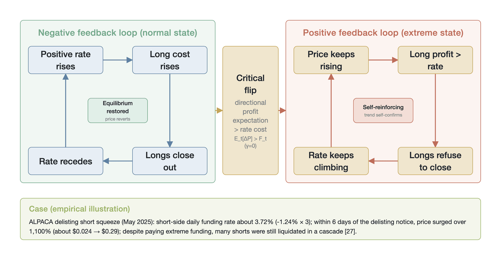
Figure 10-13. The flip of the funding rate mechanism from negative to positive feedback (a mechanism illustration based on a conceptual process, not empirical data; in the ALPACA event, −1.24%/8h is the peak negative rate, the daily total of 3.72% is extrapolated over three periods, and the price range of $0.024 to $0.29 is a conservative figure [27])
As Figure 10-13 shows, the flip proceeds in clear stages. In the normal state, a contract premium induces a positive rate, the rate cost suppresses longs and attracts arbitrageurs, forming a negative feedback loop of price convergence. Once the expected directional profit exceeds the rate cost, holders no longer close positions under rate pressure; instead, the rising rate is read as confirmation of trend continuation, drawing in more same-direction capital and flipping negative feedback into positive feedback. In the ALPACA event, this flip completed within six days of the delisting announcement, accompanied by a price increase of more than 1,100% and chain forced liquidations of shorts [27].
10.5.2 A behavioral finance explanation
In the positive-feedback phase, the market exhibits a counterintuitive phenomenon: "the higher the funding rate, the more the paying side refuses to close." Beyond the pure mathematical profit calculation above, the behavioral-finance research of scholars such as Skwarek (2025) offers a deeper explanation for such irrational behavior in the crypto market [28].
The sunk cost fallacy and the disposition effect are the primary factors. After paying substantial funding rates and enduring paper losses, traders are often unwilling to accept the loss and exit. The disposition effect shows that investors tend to sell winning assets too early and hold losing assets too long. In a high-rate environment, closing a position means converting the paper loss and the rate already paid into a realized loss, and this psychological pain leads traders to keep holding. Confirmation bias reinforces the same behavioral pattern. In a polarized market, traders tend to selectively seek information supporting their position direction while ignoring the risk signal sent by a high funding rate. For example, at a bull-market peak, longs rationalize the extreme positive rate they pay with narratives of institutional entry or technical breakouts. Herding intensifies this dynamic further. The crypto market has pronounced social and community-driven characteristics. When the funding rate is extremely skewed to one side, it actually reflects the highly homogeneous expectations of market participants. Retail traders often believe the crowd's judgment is more accurate and thus establish positions in the crowd's direction, further intensifying rate polarization. At the theoretical level, two herding mechanisms must be distinguished: the rational information cascade described by Banerjee (1992) [29], in which each trader infers others' private information from their behavior and rationally imitates it, versus pure social conformity. The on-chain position transparency of the crypto market (such as Hyperliquid's public whale-position leaderboard) significantly accelerates the information-cascade effect by lowering the cost of observing behavior: traders can observe the direction and size of large positions almost in real time, which has no direct counterpart in the traditional-finance herding literature. Together, these factors point to gambling-like sensation-seeking behavior; Delfabbro and colleagues note that the behavior of some crypto traders is structurally similar to pathological gambling [30]. The extreme high-leverage, high-rate environment not only fails to deter but instead provides the high volatility and thrill they seek.
10.5.3 Termination paths of polarization
Once the funding rate falls into a polarized positive-feedback loop, it usually terminates in only one of two ways, whose effects on market structure differ starkly. Along the two dimensions of leverage concentration and liquidity depth, Figure 10-14 compares the two termination paths of polarized positive feedback: mild mean reversion and liquidation cascade.
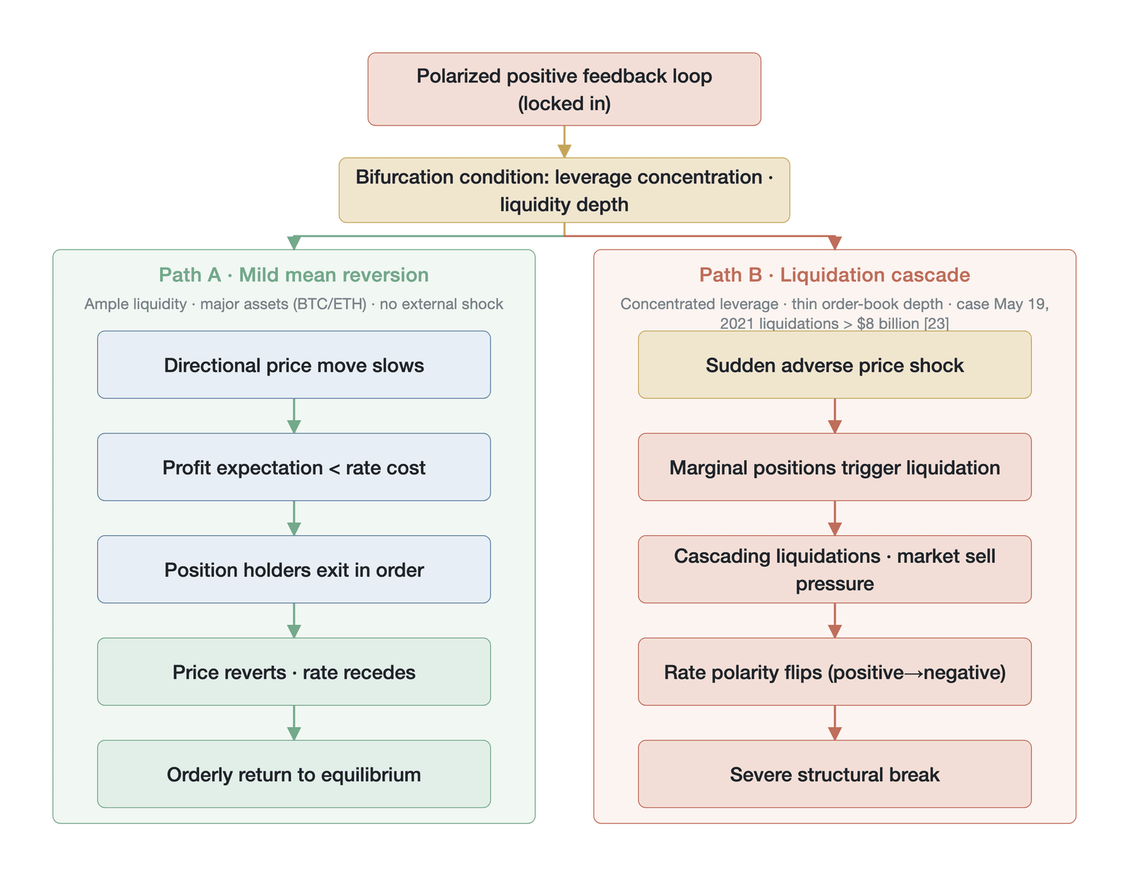
Figure 10-14. A comparison of the two termination paths of funding rate polarization positive feedback (a conceptual illustration based on synthetic trajectories, not empirical data)
In the case of mild mean reversion, the one-sided movement of the asset price begins to slow or stall, the expected directional profit falls accordingly, and the mathematical trigger condition reverses (expected profit < rate cost). Holders realize that continuing to pay a high rate is no longer worthwhile and begin to close positions actively, in an orderly, staged manner. As one-sided positions decline, the contract price moves back toward the spot price and the funding rate gradually falls to normal levels. This path usually occurs in mainstream assets with good liquidity and ample arbitrage capital (such as BTC and ETH), absent a major external macro shock.
By contrast, the liquidation cascade path is far more destructive. When polarized one-sided positions (usually accompanied by high leverage) encounter a sudden adverse price move, some marginal positions are triggered into forced liquidation. In the case of positive-rate polarization (a crowded long side), long liquidations generate large numbers of market sell orders that instantly depress the contract price, in turn triggering long stop-losses and liquidations at lower price levels. This chain of forced long liquidations drives the contract price far below the spot price in a very short time, and the funding rate not only instantly returns to zero but may even flip polarity, from an extreme positive rate to an extreme negative rate. The crash of May 19, 2021 is a canonical case: more than $8 billion in leveraged longs were liquidated within about 24 hours, and the funding rate fell from a sustained high positive value to an extreme negative value [23].
10.5.4 Rate polarization and the leverage cycle
Rate polarization is not an isolated event; it is the crypto derivatives market's counterpart to Hyman Minsky's "financial instability hypothesis" [31]. Minsky argues that prolonged stability breeds overconfidence, which in turn drives the accumulation of debt leverage and ultimately leads to collapse (the "Minsky moment").
The mapping is not exact, and its limits are worth stating precisely. The core causal chain of the Minsky framework is the gradual deterioration of the debt-to-income ratio and the hard constraint of repaying principal at maturity. Perpetual futures holders face no maturity-repayment constraint, and what triggers deleveraging is not "cash flow failing to cover interest" but the forced liquidation of margin. This changes the temporal profile of the crisis: the traditional Minsky cycle is gradual (usually unfolding over months to years of leverage accumulation), whereas a liquidation cascade in the crypto market can complete within minutes, so the transition from "boom" to "bust" is several orders of magnitude faster. The crypto market's leverage cycle is therefore more accurately described as an "accelerated Minsky," which retains the leverage-driven positive-feedback core while compressing the unfolding of the crisis from the quarterly scale of the macroeconomy to the minute scale of the microstructure.
In the crypto market, the evolutionary trajectory of the funding rate exhibits a close mapping to the leverage cycle. Figure 10-15 decomposes this mapping into four phases: leverage accumulation, criticality, deleveraging, and recovery.
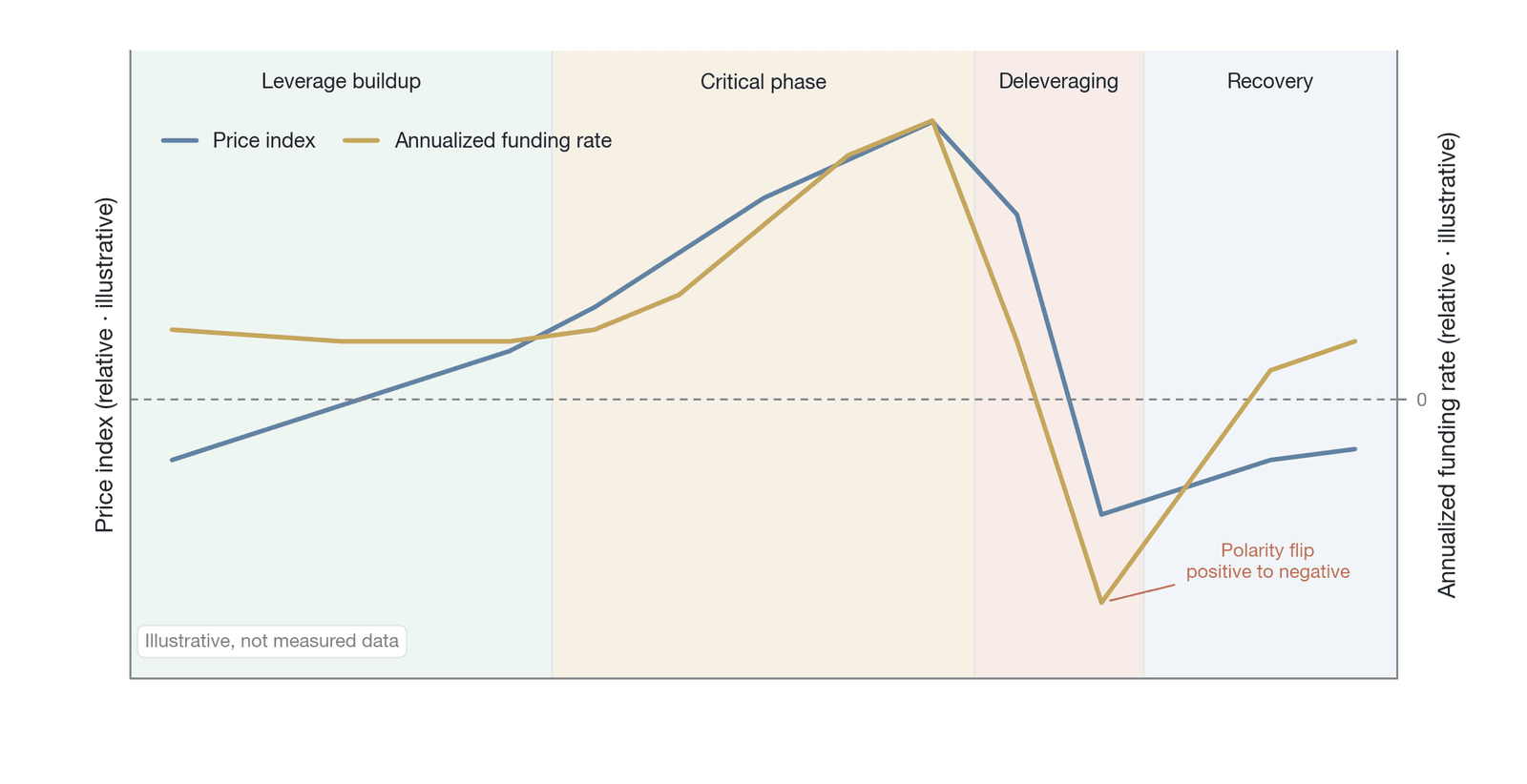
Figure 10-15. The mapping between the crypto-market leverage cycle and the evolution of the funding rate (a conceptual illustration, not empirical data; the horizontal axis shows qualitative cycle phases and the vertical axis shows relative levels, not measured scales)
The leverage accumulation phase (hedge finance) marks the start of the cycle: the market rises steadily, the funding rate stays at a mild positive value slightly above 0.01%, arbitrageurs participate actively, and the market appears to be in a stable equilibrium. As the market advances, it enters the criticality or euphoria phase (speculative and Ponzi finance). Prices accelerate upward, speculators use paper profits to add positions and become desensitized to the rate cost. The funding rate soars and stays elevated, arbitrageurs' capital is exhausted, and negative feedback flips into positive feedback. At this point, an extreme funding rate is a clear signal that market leverage is over-concentrated and the system is highly fragile. When this fragility peaks, it triggers the deleveraging phase (the Minsky moment). A small external shock can set off a liquidation cascade, causing a price collapse. The funding rate flips polarity, from positive to negative, deeply reflecting the market's panic and liquidity drought. After violent turmoil, the market finally enters the recovery phase. Leverage is thoroughly washed out, the market enters a low-volatility phase, and the funding rate slowly returns toward zero or its default benchmark, quietly awaiting the gestation of the next cycle.
A persistently polarized funding rate is therefore not only a cost indicator but also a state variable measuring the market's systemic risk and leverage fragility. In practice, quantitative traders and risk managers can incorporate the duration and magnitude of rate polarization into early-warning models: when the funding rate stays above its historical 90th percentile for more than 48 hours, the market is in a high-probability window for a deleveraging event. Section 10.8 tests this hypothesis systematically and empirically.
10.5.5 The reconfiguration of participant behavior
When the market enters an extreme rate environment, the original three-layer game ecosystem breaks down, and the behavioral patterns and risk-return profiles of each participant are reconfigured. Figure 10-16 compares the changes in profit impact and risk exposure of five participant types under an extreme rate environment, revealing the transition from an arbitrageur-dominated orderly equilibrium to a liquidator-dominated disorderly state.
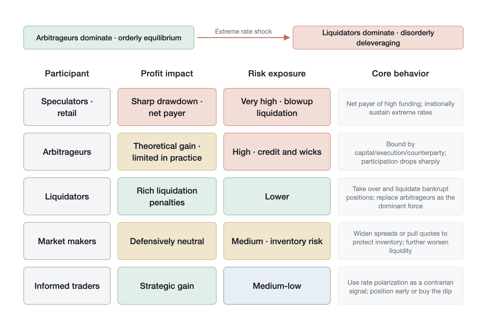
Figure 10-16. The reconfiguration of profit impact and risk exposure for each type of participant under an extreme funding rate environment (an illustrative relative assessment, not empirical data; the relative impact is assigned by the author)
Speculators and retail traders come under pressure first in rate polarization, becoming the net payers of the high rate, facing the largest profit drawdown and extremely high liquidation-risk exposure; their irrational persistence is precisely the driver that sustains the extreme rate. At the same time, the position of rate arbitrageurs also changes subtly. Although they can in theory earn excess rate income, they are constrained by the three boundaries of capital, execution, and counterparty, so their actual participation declines sharply, and they instead must bear extremely high exchange credit risk and wick risk. In this environment, liquidators replace arbitrageurs as the dominant market force. They earn substantial liquidation-penalty income by taking over and liquidating bankrupt positions, at relatively low risk. Market makers' behavior further aggravates the turmoil: amid violent fluctuations, they typically widen the bid-ask spread or pull orders outright to protect their inventory, which further worsens liquidity and intensifies the extremes in price and rate. By contrast, informed traders act more strategically. They use rate polarization as a contrarian indicator, positioning in the opposite direction ahead of a violent liquidation cascade, or providing liquidity to buy the dip after a cascade occurs.
In sum, the flip of the funding rate from negative to positive feedback marks a state transition of the market microstructure from orderly arbitrage to disorderly deleveraging. Understanding this polarization process directly informs the design of resilient crypto-asset trading strategies and risk-management frameworks.
10.6 The spectrum of strategic behavior
The funding rate mechanism was originally designed to anchor perpetual futures to spot prices, but in actual operation this mechanism inevitably breeds a complex game around its rules. Market participants are no longer merely price-takers but players of the mechanism. As the derivatives market's microstructure has matured, trading strategies around the funding rate have grown from simple cash-and-carry arbitrage into a full spectrum of more complex behaviors. This section systematically reviews this strategy spectrum and, through data and empirical cases, analyzes the impact of different strategies on market equilibrium and the internal logic of their evolution toward systemic manipulation.
10.6.1 A three-tier classification
By their contribution to market pricing efficiency and their manner of exploiting trading rules, funding-rate-related trading strategies can be divided into three tiers, forming a continuous spectrum from compliant arbitrage to systemic manipulation. Figure 10-17 arranges these three tiers along the two dimensions of compliance and market impact.
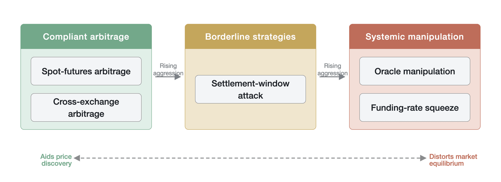
Figure 10-17. The spectrum of funding rate strategic behavior
The first tier is compliant arbitrage, mainly comprising traditional cash-and-carry arbitrage and cross-exchange rate arbitrage (the specific operating mechanisms of both are described in Section 10.4.2). These strategies earn rate income while bearing very low market risk, supply important liquidity, and perform the core function of eliminating price deviations and promoting price discovery, all of which supports the healthy functioning of the market.
The second tier comprises edge strategies. These strategies begin to operate in the gray area of the rules, their main feature being to profit by exploiting microstructural flaws in the mechanism design. A typical edge strategy is the "settlement window attack." Under a fixed-time settlement mechanism (such as traditional 8-hour settlement), a trader closes positions a few seconds before settlement to avoid the rate payment and re-establishes them immediately afterward. Although this behavior does not violate the trading rules, it causes severe liquidity fluctuations during the settlement window and reduces the effectiveness of the funding rate's anchoring mechanism.
The third tier is systemic manipulation. When edge strategies combine with a specific market structure (such as low liquidity and high concentration), they can evolve into systemic manipulation. Systemic manipulation no longer passively exploits rate differences but actively controls the spot or contract price to artificially create an extreme funding rate environment, forcing counterparties to be liquidated because they cannot bear the enormous funding cost or run out of margin. Typical systemic manipulation includes oracle manipulation and rate squeezes. In these strategies, the funding rate has been transformed from a tool for maintaining price anchoring into a tool for attacking counterparties. This chapter treats rate squeezes as game-theoretic cases for descriptive analysis, but such behavior may legally constitute market manipulation. In traditional securities markets, using an information advantage to control supply and engineer a forced-liquidation cascade in the derivatives market is a criminal offense in most jurisdictions. The U.S. Department of Justice filed criminal charges against Avraham Eisenberg in January 2023 (commodities fraud, commodities manipulation, and wire fraud), with the CFTC and SEC filing parallel civil enforcement actions at the same time; in April 2024 a jury found him guilty on three counts [32] (the criminal conviction was vacated in May 2025 by a federal judge on grounds including venue, and prosecutors have appealed). This shows that such behavior faces substantial enforcement risk in the digital-asset market, even though its ultimate legal characterization remains uncertain. In addition, an exchange's changing the settlement frequency during the life of a contract (such as the shift from 8 hours to 1 hour in the ALPACA event) constitutes, under contract-law frameworks, a unilateral modification of a core contractual term. Although an exchange's terms of service usually reserve such modification rights, their legal validity and their legitimacy with respect to user interests remain contested across jurisdictions.
10.6.2 Equilibrium characteristics under normal markets
In a normal market where no systemic manipulation occurs, the funding rate exhibits specific statistical distribution characteristics. These characteristics reflect the equilibrium state of market participants within a compliant-arbitrage framework. Through a statistical analysis of 2,190 8-hour settlement rate data points for Binance's BTCUSDT perpetual futures from January 2024 to December 2025 (, excluding the data points generated at higher frequencies during the 2025 dynamic-settlement-frequency period), we can clearly observe this equilibrium characteristic.
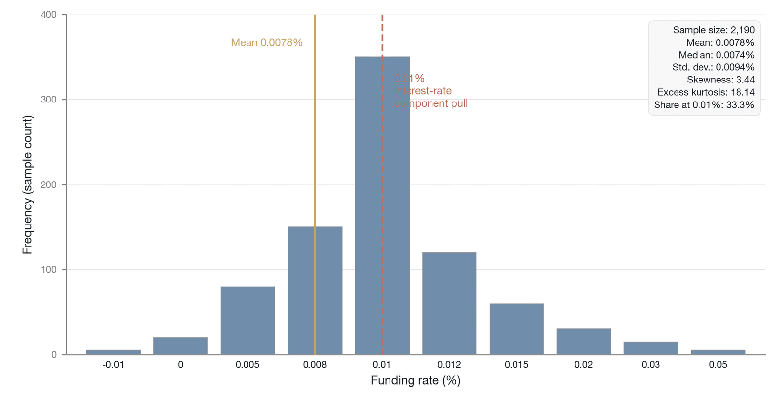
Figure 10-18. The distribution characteristics of BTCUSDT perpetual futures funding rates (computed by the author from the Binance BTCUSDT 2024–2025 funding rate history; descriptive statistics; the histogram is drawn in equal-width bins with stylized bar heights, and the excess kurtosis is highly sensitive to extreme observations)
As the figure above shows, the funding rate distribution under normal conditions has a pronounced leptokurtic (sharp-peak, fat-tail) character. The data's excess kurtosis reaches 18.14, far above the normal-distribution baseline of 0 (corresponding to a raw kurtosis of 21.14). This means the funding rate is highly concentrated at a specific level most of the time but occasionally exhibits extreme deviations. Note that the funding rate time series has a significant autocorrelation structure (volatility clustering), and the excess kurtosis of 18.14 may be partly attributable to this time dependence rather than to true fat tails under an i.i.d. assumption. After removing the autocorrelation structure (for example, via GARCH filtering), the excess kurtosis of the residuals may decline somewhat but still deviate significantly from normality.
Moreover, the distribution of the funding rate is markedly right-skewed (skewness of 3.44), with a mean of 0.0078%, slightly above zero. This structural positive deviation reflects the long-standing long premium in the cryptocurrency market. Because market participants generally tend to use leverage to go long, the contract price is often above the spot price, and longs must pay shorts the funding rate.
The data show one more prominent feature: in fully 33.3% of all samples, the funding rate stays exactly at 0.01%. This phenomenon is not the result of natural market trading but a direct expression of the "interest rate component" in the mechanism design. In Binance's older formula, the base rate was fixed at 0.03% per day (i.e., 0.01% every 8 hours), and when the market premium was within the clamp band, the funding rate was dominated by this fixed rate. This "gravitational effect" shows that under normal conditions, the mechanism rules often determine the rate more than actual market supply and demand do.
10.6.3 The ALPACA funding rate squeeze case
When fragility appears in the market microstructure, the normal equilibrium is broken and the funding rate can become a tool for systemic manipulation. The ALPACA rate squeeze that occurred on Binance in April–May 2025 is a canonical case of this phenomenon. The event exhibited the contract paradox of "a negative catalyst triggering an extreme positive price reaction."
On April 24, 2025, Binance announced that it would delist the ALPACA spot trading pair on May 2 and settle the perpetual futures on April 30. In traditional market logic, a delisting announcement is a strong bearish signal. This news quickly formed a consensus expectation among retail traders that "the price will inevitably go to zero," causing large amounts of short capital to pour into ALPACA perpetual futures and forming an extremely crowded short camp.
The manipulator, however, recognized this structural weakness. At the time, ALPACA's circulating market capitalization had shrunk to about $5 million, and the token was highly concentrated. The manipulator used very little capital to buy continuously in the spot market, driving up the spot price, while establishing long positions in the contract market. Because of the large presence of shorts, the contract price was severely depressed, causing the funding rate to take an extreme negative value (shorts paying longs).
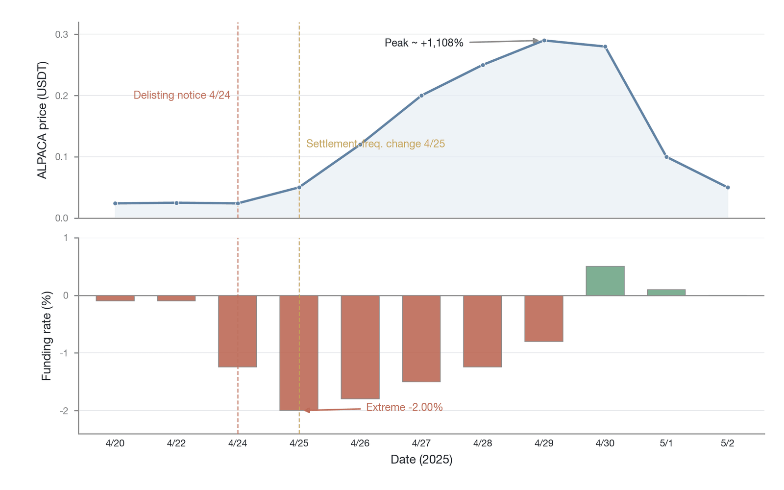
Figure 10-19. Price and funding rate movements during the ALPACA funding rate squeeze (illustrative movements, event reconstruction); the price range of $0.024 to $0.29 is a conservative figure, the rate cap moved from ±2% to ±4%, and the total liquidations of about $50 million (of which about $43 million were shorts) have been verified value by value [27]
As the figure above shows, after the delisting announcement, the ALPACA price did not crash but instead surged violently, with a peak gain of more than 1,100%. At the same time, the funding rate hit its floor deeply. To respond to the extreme market conditions, Binance activated the dynamic settlement-frequency mechanism on April 25, gradually shortening ALPACA's settlement frequency from every 8 hours to every 1 hour and adjusting the rate cap to ±2% (and subsequently widening it to ±4%).
This mechanism adjustment was intended to raise the cost of manipulation, but objectively it sharply accelerated the depletion of short margin. Under 1-hour settlement and a ±2% rate cap, a short position had to pay as much as 2% in funding every hour, amounting to a daily cost as high as 48% (this calculation applies to the old algorithm before the September 2025 normalization update. The ALPACA event occurred in April–May 2025, when Binance had not yet introduced the frequency normalization factor; note also that the rate is calculated on the notional position value, and because the ALPACA price rose more than 1,100% during this period, the absolute amount of each later period's rate was far larger than that of the early periods, a nonlinear amplification effect). At this rate level, the funding rate is no longer a marginal trading cost but a cash-flow burden the holder cannot bear. Facing enormous funding costs and a continuously rising price, shorts were forced to close (buy), and this chain of forced short liquidations pushed the price higher still, ultimately producing total liquidations of about $50 million (of which about $43 million were shorts). In this case, the actual effect of the funding rate mechanism ran counter to its corrective intent, becoming a tool for the manipulator to amplify counterparty losses.
From the ALPACA case, we can distill a more general model of rate-manipulation feasibility. The manipulator's expected profit can be expressed as:
where is the gain from squeezing the counterparty (including the price-impact profit from the counterparty's forced closing and the rate income), is the capital cost of establishing and maintaining control in the spot market, and is the funding-rate outlay the manipulator's own side bears over the manipulation period. This simplified model omits nonlinear execution costs: on an extremely thin order book, the manipulator's position-building self-inflates the price, and the closing slippage of the squeezed shorts amplifies actual losses; a more complete model should add a market-impact function (such as the Almgren-Chriss framework) to capture these nonlinear frictions. Even so, the feasibility of manipulation still depends on three key parameters: the circulating market capitalization M (the lower M, the smaller ), the short concentration ρ (the higher ρ, the larger , because crowded shorts are more easily liquidated in a chain), and the settlement frequency f (under the un-normalized old algorithm, the higher f, the faster the counterparty's cumulative rate burden grows). ALPACA happened to satisfy all three conditions simultaneously—low M (circulating market capitalization of about $5 million), high ρ (delisting expectations made shorts extremely crowded), and high f (Binance raised the settlement frequency from 8 hours to 1 hour)—making the expected profit of manipulation far exceed its cost. This framework indicates that in assessing a token's manipulation risk, regulators and exchanges should systematically monitor the combined state of these three parameters.
The ALPACA event and similar high-frequency-settlement squeezes exposed a systemic vulnerability in early funding rate mechanisms under extreme conditions. In particular, when the settlement frequency is dynamically raised, if the calculation of the per-settlement rate remains unchanged, the daily cumulative rate cost is amplified many times over, giving manipulators an opening.
To patch this vulnerability, Binance made a major update to the funding rate formula on September 18, 2025. The core of this update was the introduction of a "frequency normalization factor."
In the old algorithm before the update, the per-settlement funding rate formula was:
where is the average premium index over the settlement period. Under the old algorithm, when the settlement frequency was shortened from 8 hours to 1 hour, although each settlement covered a shorter time, the part of the formula determined by the premium index did not scale down proportionally. This means that if the market has a persistent extreme premium, the per-settlement rate under 1-hour settlement can be of the same order of magnitude as the per-settlement rate under 8-hour settlement, amplifying the daily cumulative rate eightfold.
The updated new algorithm introduces the frequency normalization factor, where N is the number of hours in the settlement period:
The logic of this formula is to first compute a nominal rate using the standard 8-hour formula, then multiply by N/8 to scale. Note that the clamp bounds (, ) do not scale with the settlement frequency in the formula; the scaling applies only to the overall result. For a concrete numerical example: assume the average premium index and the interest rate component I = 0.01%. When N = 8 (the old algorithm), , and the daily cumulative rate is ; when N = 1 (the new algorithm with 1-hour settlement), , and the daily cumulative rate is —the two daily cumulative rates are exactly identical.
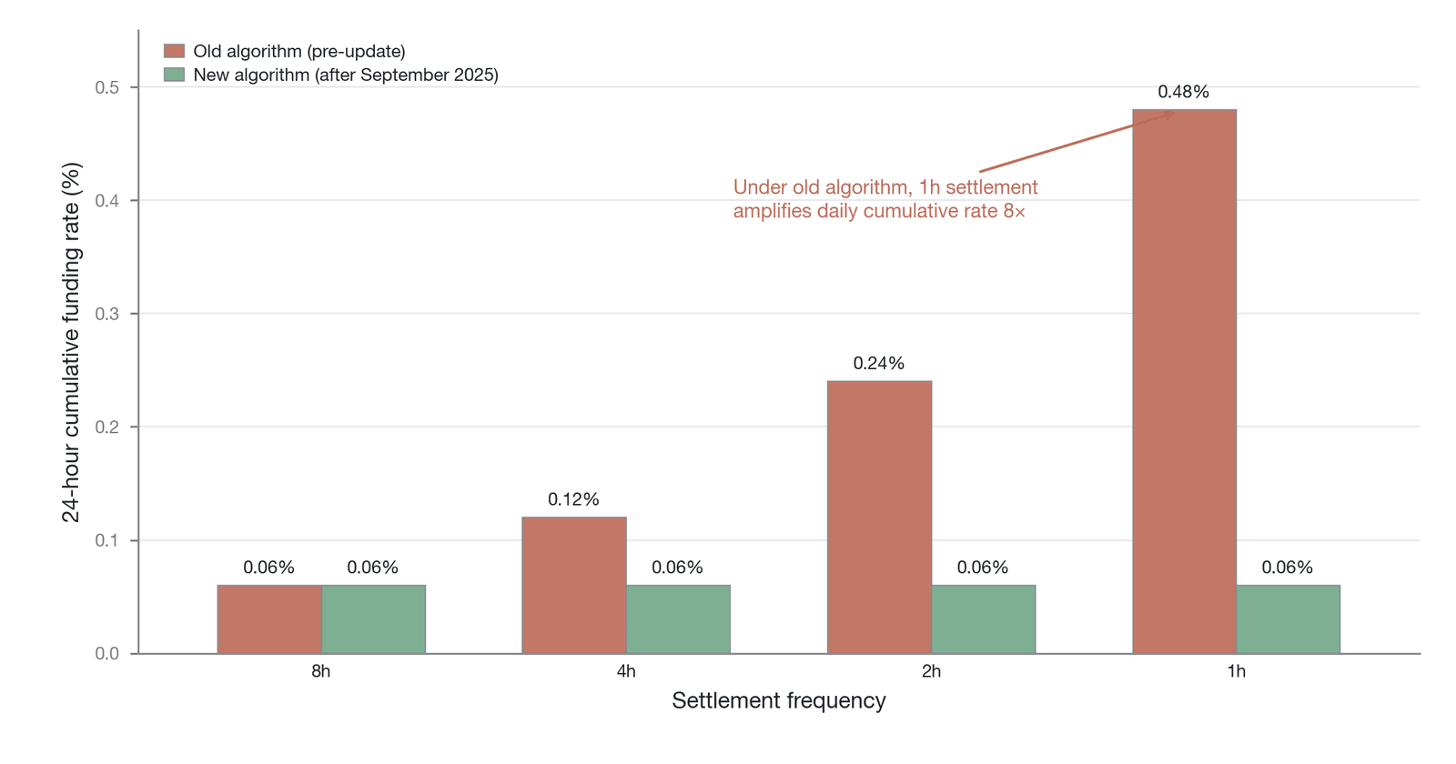
Figure 10-20. A comparison of daily cumulative rates before and after Binance's funding rate algorithm update (a formula-derived illustration with a real mechanism; the example values are constructed and are not the 0.45%/1.35% worked example in the main text [10])
As Figure 10-20 shows, by introducing the frequency normalization factor, the new algorithm ensures that at the same market premium level, regardless of how the settlement frequency changes (8 hours, 4 hours, 2 hours, or 1 hour), the theoretical upper bound of the cumulative funding rate over 24 hours remains consistent. This mechanism evolution effectively seals off the attack path by which manipulators used high-frequency settlement to amplify counterparty costs, and it is a concrete improvement of the funding rate mechanism toward manipulation resistance. Binance also shortened the calculation baseline of the mark price from 1 minute to 30 seconds, improving the system's responsiveness to abnormal price fluctuations and further compressing the space for manipulation.
10.7 The settlement frequency game
In the early design of perpetual futures, the settlement frequency of the funding rate was usually static and fixed (such as every 8 hours). This design had advantages in reducing the system's computational load and providing predictability. As market volatility increased and strategies grew more complex, however, static settlement frequency gradually revealed its fragility under extreme market conditions. Beginning in 2025, major exchanges successively introduced dynamic settlement-frequency mechanisms, a shift that is less a technical upgrade than a change in mechanism-design philosophy, from passive reaction to active management.
10.7.1 From passive reaction to active management
The traditional 8-hour static settlement mechanism is essentially a "passive reaction" system. It assumes that the market has enough time (8 hours) to digest information and restore equilibrium, with the funding rate serving merely as a mild corrective tool. In the crypto market, however, asset prices can fluctuate violently within minutes, and an 8-hour settlement period means the system is in a "blind spot" most of the time, providing ample room for edge strategies such as the settlement window attack.
The introduction of the dynamic settlement-frequency mechanism marks the beginning of exchanges adopting an "active management" posture. Take the dynamic mechanism that Binance fully implemented in May 2025: the system automatically switches the settlement frequency among 8 hours, 4 hours, and even 1 hour according to the real-time state of the market premium. Binance's dynamic settlement-frequency mechanism is not fully algorithmic, however: the decision to switch frequency involves a manual or semi-automated approval step, and the trigger condition depends not only on the rate itself but also on a multidimensional assessment of the absolute value of the premium index, its duration, and the overall market risk situation. The mechanism's transition "from passive to active" therefore spans two levels—algorithmic automation and human risk-control judgment—and the latter has inherent limitations in transparency and predictability.
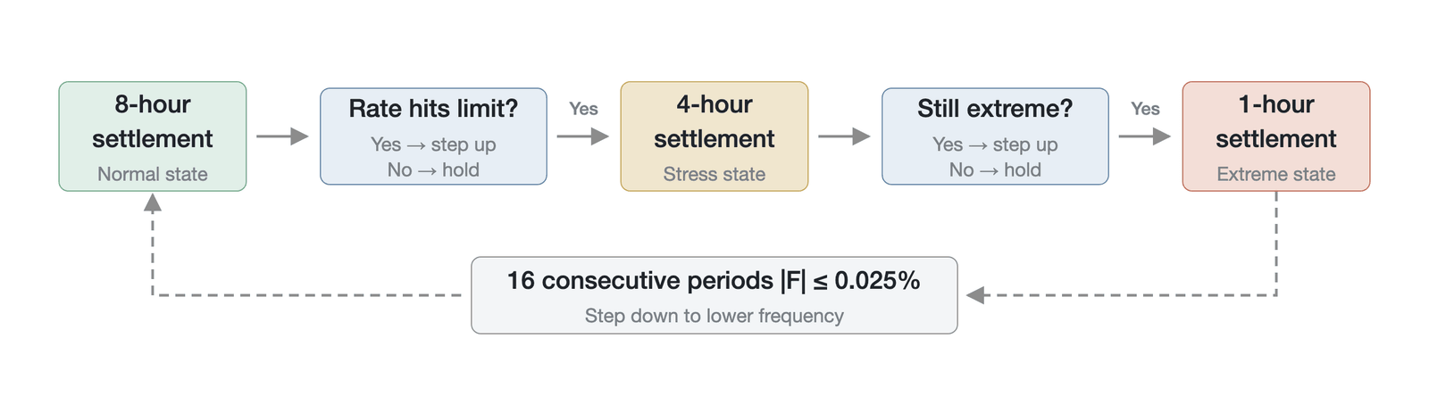
Figure 10-21. The state-transition logic of the dynamic settlement frequency mechanism (a mechanism illustration; the recovery threshold of 16 consecutive periods with |rate| ≤ 0.025% is the author's illustrative rendering of the mechanism's logic, not a published specification)
As Figure 10-21 shows, the core logic of the mechanism is that when the funding rate repeatedly hits the set upper and lower bounds, the system automatically raises the settlement frequency (for example, from 8 hours to 4 hours, then to 1 hour). Only when the market returns to calm (for example, when the absolute value of the funding rate is less than or equal to 0.025% for 16 consecutive periods) does the system gradually restore a lower settlement frequency. This design turns the settlement frequency itself into an endogenous game variable, enabling the mechanism to adaptively adjust the strength of correction according to market stress.
10.7.2 The game-theoretic implications of different settlement frequencies
Different settlement frequencies have starkly different game-theoretic implications for participant behavior and market microstructure. Table 10-7 compares in detail the market characteristics under three main settlement-frequency modes:
| Dimension | 8-hour static settlement | 1-hour high-frequency settlement | Continuous settlement |
|---|---|---|---|
| Arbitrageur behavior | Concentrated around settlement (settlement window attack), causing periodic liquidity fluctuations | Trading is distributed more evenly, arbitrage opportunities are fleeting, and high automated-trading capability is required | Arbitrage behavior is fully smoothed, eliminating the traditional settlement window attack, but the EMA reference window it relies on (such as dYdX v4's 8-hour EMA) itself creates a new microstructural manipulation dimension, as an instantaneous price shock can affect the rate throughout the entire EMA window |
| Funding cost accumulation | Step-wise jumps; each payment is large in amount, but there is ample time to close and avoid it | Rapid accumulation; continuous cash-flow pressure; high holding cost | Real-time interest accrual; continuous deduction; extremely high margin requirements |
| Suppression of one-sided markets | Weaker; within 8 hours the price may already have deviated irreversibly | Stronger; the high holding cost forces the disadvantaged side to surrender quickly | Extremely strong; a price deviation is immediately converted into a cash-flow penalty |
| System-performance requirements | Low; suitable for large-scale concurrent computation | Higher; requires more frequent snapshots and liquidations | Extremely high; usually implemented only on-chain in perpetual futures protocols or specific architectures |
Table 10-7. Comparison of the game-theoretic implications of three settlement-frequency modes (Data source: compiled by the author)
Under the old algorithm system, because of the lack of frequency normalization, 1-hour settlement not only increased the frequency of payments but also amplified the cumulative funding cost many times over (with a premium index of 0.5%, under the old algorithm 1-hour settlement amplified the daily rate about eightfold; the mechanism and worked example are given in Section 10.6.3). Even after the introduction of the normalization factor, high-frequency settlement still significantly changes the game equilibrium between longs and shorts by increasing friction costs and reducing decision time. The compression of decision time forces trend traders to set tighter stop-losses, because the faster depletion of margin means that a countertrend position that could originally be held for several days may hit the liquidation line within hours under 1-hour settlement.
10.7.3 The PIPPIN case analysis
The PIPPIN perpetual futures event of December 2025 is a canonical case of how a high-frequency-settlement mechanism reshapes the long-short game under extreme conditions. As an emerging AI-agent-themed token, PIPPIN attracted large amounts of short capital trying to "call the top" as its price climbed rapidly and repeatedly set new highs (a closing high of about $0.54 within December). Because shorts were overcrowded, the perpetual futures price fell far below the spot price, triggering Binance's dynamic settlement mechanism and adjusting the settlement frequency to once every hour.
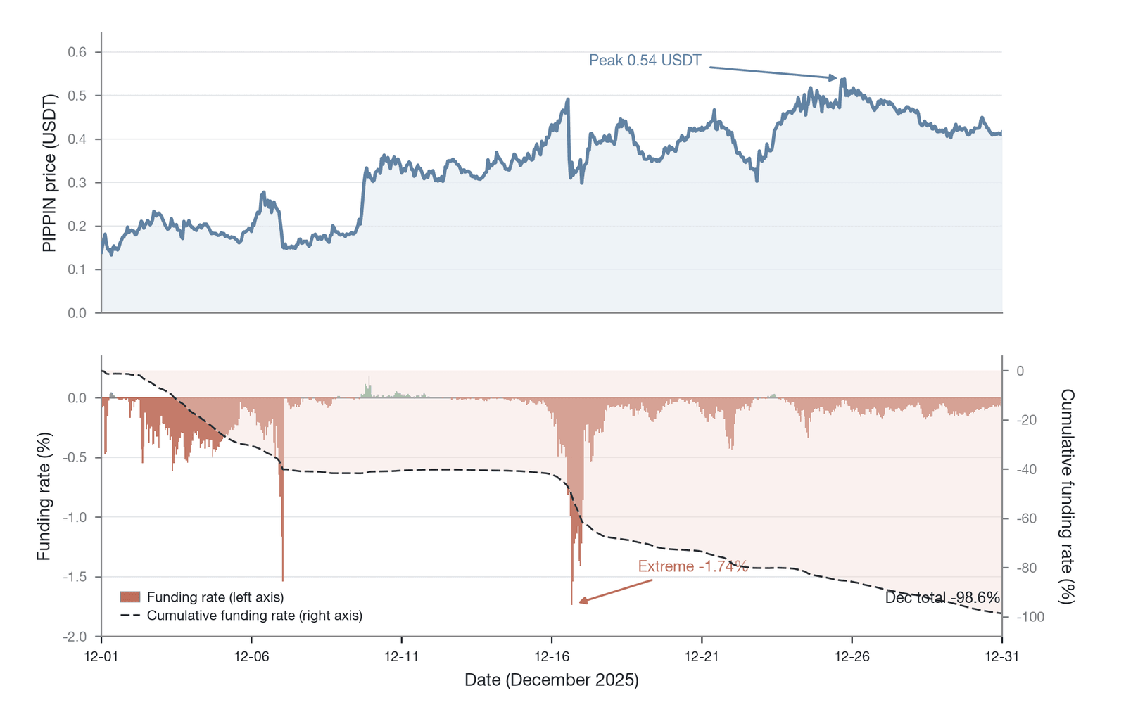
Figure 10-22. Price and funding rate dynamics for PIPPIN under extreme conditions (Data source: Binance PIPPINUSDT perpetual, 1-hour settlement, hourly observations for December 2025; as of June 30, 2026; the extreme single-period rate within the month was −1.74%, and the cumulative funding rate for the full month was about −98.6%)
As Figure 10-22 shows, during the extreme conditions of mid-December, PIPPIN's funding rate stayed for a long time in a deeply negative range. In particular, from December 16 to 17, there were dozens of hours of continuous high negative rates. According to live data, in the most extreme 24 hours (18:00 on December 16 to 17:00 on December 17), a short position's cumulative funding-rate outlay was as high as −19.77%. Over the whole of December, PIPPIN experienced 26 consecutive high-negative-rate cycles, the longest lasting 80 hours, during which the cumulative funding rate reached −27.81%.
Such high-frequency, high-magnitude funding rates dealt a devastating blow to shorts. For a trader holding a short with a notional value of about 3.53 million USDT, one day's funding-rate outlay alone could approach 700,000 USDT.
From the operational-risk dimension, the PIPPIN event also exposed two problems that are easily overlooked but critically important for live trading in a high-frequency-settlement environment. The first is liquidation-engine pressure: when large numbers of shorts trigger forced liquidation simultaneously, the liquidation engine must execute large numbers of buy market orders in a very short time, placing extreme pressure on order-book depth and matching-system throughput and potentially causing shortfall losses and accelerated insurance-fund depletion. The second is the margin-management dilemma: under an hourly deduction mechanism, traders face multiple execution dilemmas including congested deposit channels, delays in cross-exchange fund transfers, and the automatic reduction of notional position size through partial liquidations. In PIPPIN's extreme rate environment, these operational-level frictions may be the decisive factor in a trader's final P&L, rather than merely a minor assumption in a theoretical model.
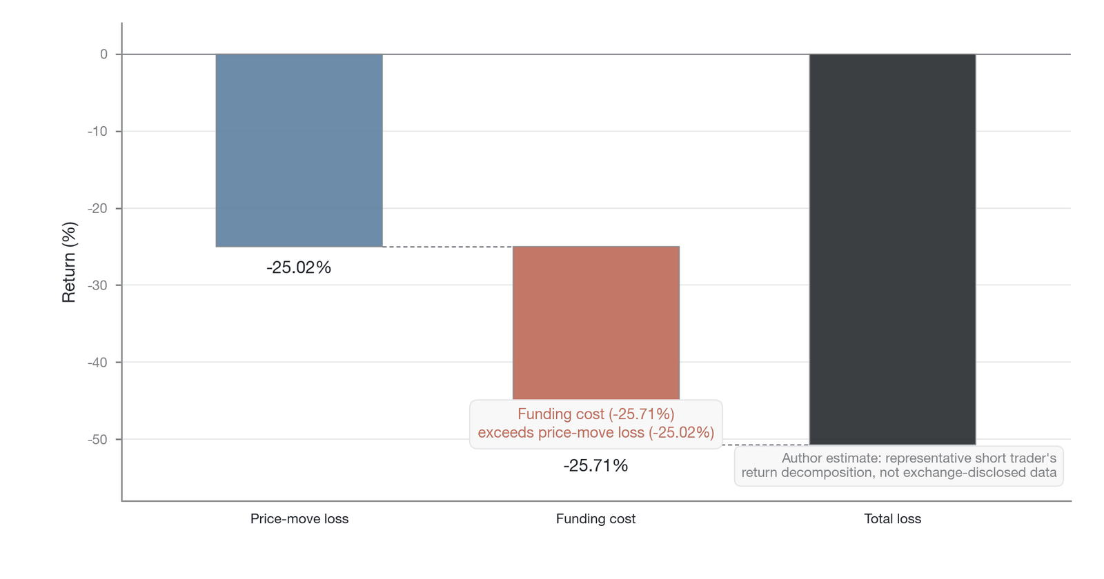
Figure 10-23. A decomposition of the return of a PIPPIN short trader (a representative/illustrative decomposition, estimated by the author, not measured from a specific account)
Through a decomposition of the return of a typical short trader (Figure 10-23), a counterintuitive pattern emerges: of the total loss of −50.73%, the loss from price movement was −25.02%, while the loss from funding-rate outlays reached −25.71%. The cost of the funding rate had exceeded the loss caused by price movement itself. This decomposition demonstrates forcefully that under a high-frequency-settlement mechanism, the funding rate is no longer a secondary friction cost but the core variable determining a trade's P&L outcome.
10.7.4 Microstructure effects of dynamic settlement
The introduction of dynamic settlement frequency has had a profound systemic impact on the microstructure of the derivatives market, and different types of participants have been forced to adjust their behavioral patterns:
Market makers and liquidity providers are directly affected: high-frequency settlement requires market makers to have stronger inventory-management capability and faster hedging speed. On on-chain derivatives DEXs, because there is no centralized risk control, market makers often must bear large unrealized profits and extremely high funding-rate outlays. This forces them to complete their pump and distribution within a very short time, or else the enormous interest outlays will rapidly erode their operating capital. The strategies of trend traders also face severe challenges. For a trend trader holding a one-sided position, the dynamic mechanism significantly increases the time cost of holding. When holding a countertrend position, high-frequency settlement accelerates the depletion of margin, so that the risk of the traditional hold-and-endure strategy rises significantly, forcing traders to stop out earlier, which may in turn intensify one-sided price movement in the short run. The survival space of arbitrageurs is likewise reconfigured. Dynamic settlement compresses the space for the settlement window attack but also creates new arbitrage opportunities based on expectations of frequency switching. Arbitrageurs must build more complex models, forecasting not only the price's return but also the state transition of the settlement frequency.
10.7.5 The costs of high-frequency settlement
Although the dynamic high-frequency-settlement mechanism demonstrates strong corrective power when addressing extreme market deviations, it is not without cost. From a game-theoretic perspective, the widespread application of this mechanism prompts deep reflection on the boundaries of market design.
The first problem is intensified liquidity friction. Although high-frequency settlement smooths the payment of funding, the frequent cash-flow transfers themselves constitute a systemic friction. When market liquidity is insufficient, a high funding rate may cause liquidity providers to exit because they cannot bear the interest cost, which in turn widens the bid-ask spread and worsens market depth.
The risk of mechanism perversion also arises. As the ALPACA and PIPPIN cases show, when the market has a structural flaw (such as low circulating market capitalization or highly concentrated holdings), the funding rate mechanism—designed to penalize deviation—may instead be exploited by manipulators to become a tool for engineering short or long squeezes. High-frequency settlement objectively shortens the disadvantaged side's reaction time and accelerates the onset of liquidation.
In sum, the settlement frequency of the funding rate is no longer a purely technical parameter but a game lever for regulating participant behavior. Future mechanism design must find a finer balance between "timely correction" and "preventing abuse of the mechanism." For example, the frequency normalization factor introduced by Binance is a successful attempt that limits the unbounded amplification of the single-day cost while retaining the deterrent power of high-frequency settlement, marking a step toward a more mature and resilient derivatives market.
From a broader mechanism-design perspective, the linear rate function currently used by most major exchanges () is not the only design choice, and its alternatives merit systematic exploration. A quadratic rate function () can impose a mild penalty for small deviations and a sharply growing penalty for large deviations, thereby strengthening corrective force under extreme states without adding friction in normal markets. A dynamic-clamp-bounds scheme allows the width of the clamp band to adjust adaptively with market volatility or open interest: narrowing the stable band in a low-volatility environment to increase the rate's sensitivity to the premium, and widening it in a high-volatility environment to prevent the rate from over-amplifying liquidation pressure. In addition, Drift Protocol (Solana) has deployed a nonlinear rate function based on the degree of long-short imbalance in open interest (rather than the price premium). This design directly targets the asymmetry of long-short open interest: even if a manipulator widens the premium by pumping the spot price, the rate does not move substantially as long as the ratio of long-short open interest does not change significantly, which in theory offers better resistance to price manipulation.
In theory, continuous settlement is the most thorough way to eliminate the time-arbitrage space of discrete settlement windows, and it brings the rate closer to a real-time feedback signal. Yet the EMA reference window it relies on introduces a new manipulation dimension. Continuous settlement faces severe engineering constraints, however. The current major on-chain perpetual futures protocols (Hyperliquid, dYdX v4) no longer run on Ethereum mainnet. Hyperliquid runs on its own L1 chain (subsecond block time, zero gas fees), and dYdX v4 is a standalone chain based on the Cosmos SDK. In these app-chain environments, the engineering constraints on continuous settlement come mainly from state consistency (all validators must reach consensus on the rate calculation at the same instant) and sequencer throughput, rather than from gas fees in the traditional sense; centralized exchanges have no such limitation, but continuous settlement requires real-time margin snapshots and equity calculations, placing far higher demands on back-end infrastructure than discrete settlement. Whether these alternatives can improve the anchoring performance and manipulation resistance of the rate mechanism while maintaining computational efficiency constitutes an open research frontier in derivatives mechanism design.
10.8 Funding rate as a state variable
In traditional microstructure analysis, the funding rate is usually treated as an output of the market state: a passive result of the imbalance between long and short forces, a friction cost the anchoring mechanism produces to correct a price deviation. When we move from the microstructural view of mechanism design to the macro view of market dynamics, however, the nature of the funding rate changes fundamentally: it is no longer merely a passive result but an information-rich state variable and a forward-looking predictor. This section advances the chapter's fifth core theoretical contribution: the funding rate as state variable hypothesis. The hypothesis holds that, because of the absolute dominance of perpetual futures in the crypto derivatives market, the funding rate not only records historical trading traces but also encodes participants' directional preferences about the future, the fragility of leverage accumulation, and the distribution of systemic risk. This shift in thinking is analogous to the paradigm evolution in traditional finance from viewing the interest rate as a passive output of monetary policy to viewing the yield curve as an active predictor of the economic outlook. The sections below deconstruct the information content of the funding rate along three dimensions—rate level, rate volatility, and the cross-asset rate surface—and draw out its fundamental differences from traditional sentiment indicators.
10.8.1 The information content of the rate level
The absolute level of the funding rate is the most intuitive signal in the market. At the first order, it conveys directional information: a positive rate means the market is net long, and a negative rate means the market is net short. The deeper value of the rate level, however, lies in its second-order information—that is, it quantifies the intensity of leverage accumulation.
Applying the three-layer decomposition model of Section 10.2, after stripping away the financing cost layer (the institutional benchmark, such as BitMEX's 0.01% every 8 hours, about 10.95% annualized) and the institutional friction layer (the truncation effect of the clamp function), the absolute value of the remaining sentiment premium layer directly measures the "overheating" of market leverage. The higher the sentiment premium layer, the deeper the leverage accumulation, and the closer the "leverage cycle" discussed in Section 10.5 is to its critical point.
In a fully efficient market, the presence of arbitrageurs should quickly return the funding rate to a neutral level. When the funding rate deviates from the neutral level for an extended period, however, it reveals the depletion of arbitrage capital or the overwhelming advantage of directional speculative force. Such a persistent deviation usually means the market is entering a fragile one-sided state. When the rate stays elevated for a long time (an extreme positive rate), longs are not only bearing a large holding cost, but the accumulation of this cost continuously erodes longs' margin buffer. This state is analogous to "potential-energy accumulation" in physics: a high rate does not directly cause a price crash, but it creates an extremely fragile system state in which any small negative shock can trigger a chain of long deleveraging. Conversely, when the rate is at an extreme negative value, shorts are paying a high price to maintain their positions, and the market is likewise extremely taut, liable to a short squeeze at any moment.
A high positive rate does not equal "market consensus bullishness"; it means only that leveraged longs are overcrowded. When crowding reaches its limit and begins to collapse, relying on the rate signal to make directional decisions faces serious risk. November 2021 is a canonical case: the funding rate of BTC perpetual futures stayed above 0.1% every 8 hours around the time the price hit its $69,000 all-time high, appearing on the surface to send a strong bullish signal; in reality, this signal reflected the over-crowding of leveraged longs rather than fundamental support. Over the subsequent two months, BTC fell more than 40%, and the long positions established during the high-positive-rate period suffered the double loss of directional loss and rate outlay. The rate mainly reflects leverage sentiment rather than a market view, and this distinction is fundamental to correctly interpreting the rate signal.
This chapter validates this mechanism with empirical data. Based on measured 8-hour funding rate data for Bitcoin and Ethereum perpetual futures on Binance from 2024 to March 2026, we divide the absolute rate value into three ranges (low rate, medium rate, high rate) and observe their power to predict rate volatility over the next 7 days.
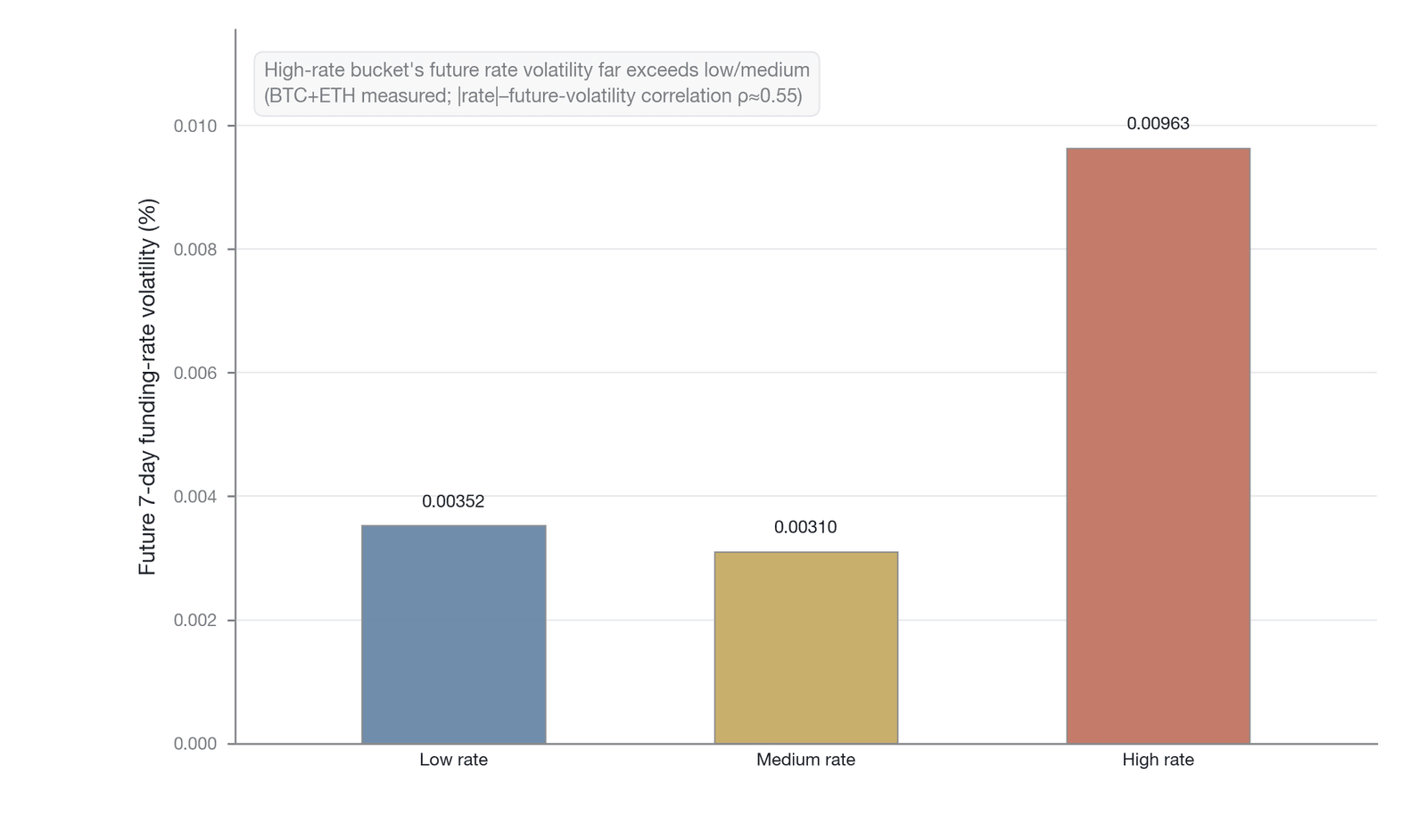
Figure 10-24. The relationship between the current absolute rate level and the funding rate volatility over the next 7 days (Data source: measured 8-hour funding rates for BTC and ETH perpetuals on Binance, 2024 to March 2026; as of June 30, 2026; the future 7-day rate volatility is averaged within tertile buckets, and the correlation between |rate| and future volatility is about 0.55)
The data show that the degree to which the current rate level is extreme is positively correlated with future volatility. When the market is in the "high rate" range (whether positive or negative), the rate volatility over the next 7 days is higher than in the "low rate" and "medium rate" ranges. This confirms that a high-rate state is essentially a high-potential-energy, high-fragility market structure: the rate level is not only a static snapshot of long-short forces but also a forward-looking indicator of future market turmoil.
10.8.2 The information content of rate volatility
If the rate level measures the degree of leverage accumulation, then rate volatility directly measures the uncertainty at the market-microstructure level and the degree of disagreement in consensus. Rate volatility is an information dimension independent of price volatility; it captures the frequency and magnitude of the swings in long-short forces within the derivatives market.
In a calm market environment, the funding rate usually fluctuates within a narrow band (dominated mainly by the benchmark rate). When the market faces a major information shock, liquidity drought, or an impeded arbitrage mechanism, however, the funding rate oscillates violently. This oscillation reflects the chaotic state of market participants repricing risk, as well as the higher risk compensation that liquidity providers (arbitrageurs) demand in the face of high volatility. Specifically:
When rate volatility is low, market consensus on direction tends to be stable. This may mean a trend has been established, or it may mean the market has fallen into complacency—the calm-before-the-storm trap. Conversely, when rate volatility is high, directional preference is switching frequently, meaning the market is full of high uncertainty. This is often a leading indicator of a market state transition (such as from trend to range, or from range to reversal). Further, a sharp rise in rate volatility is a clear signal that the market is entering a new state, analogous to a jump in VIX in traditional markets, but it more directly reflects the sudden change in uncertainty within the leveraged market.
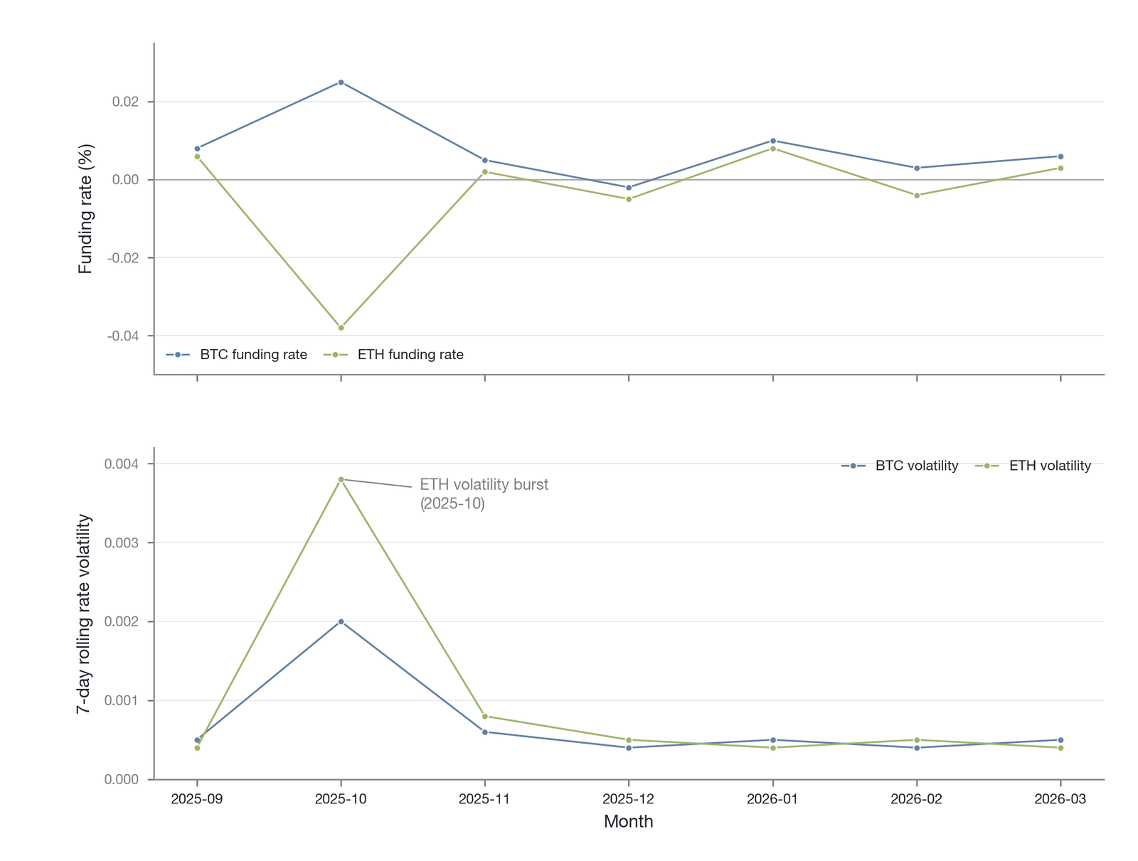
Figure 10-25. Time series of BTC and ETH funding rates and 7-day rolling rate volatility (computed by the author from the Hyperliquid API; descriptive; sample period September 2025 to March 2026, single exchange) [33]
As Figure 10-25 shows, the rate volatility of BTC and ETH is not uniformly distributed but exhibits pronounced episodic clustering. In particular market phases, rate volatility suddenly spikes, usually accompanied by violent spot-price movements or major macro events. ETH's rate volatility is significantly higher than BTC's in several periods, reflecting the structural feature of relatively shallower arbitrage depth and relatively stronger speculative force in the ETH derivatives market.
At a deeper level, a rise in rate volatility often signals a weakening of the "anchoring strength" discussed in Section 10.3. When arbitrage capital retreats because of risk aversion or capital constraints, even a small change in speculative force can cause large ripples in the rate. Rate volatility can therefore be viewed as an inverse indicator of the effectiveness of the arbitrage mechanism: the higher the volatility, the more fragile the arbitrage mechanism and the more vulnerable the market is to one-sided force.
To further quantify the impact of an extreme rate state on subsequent market behavior, we analyze the change in market activity after extreme-rate days.
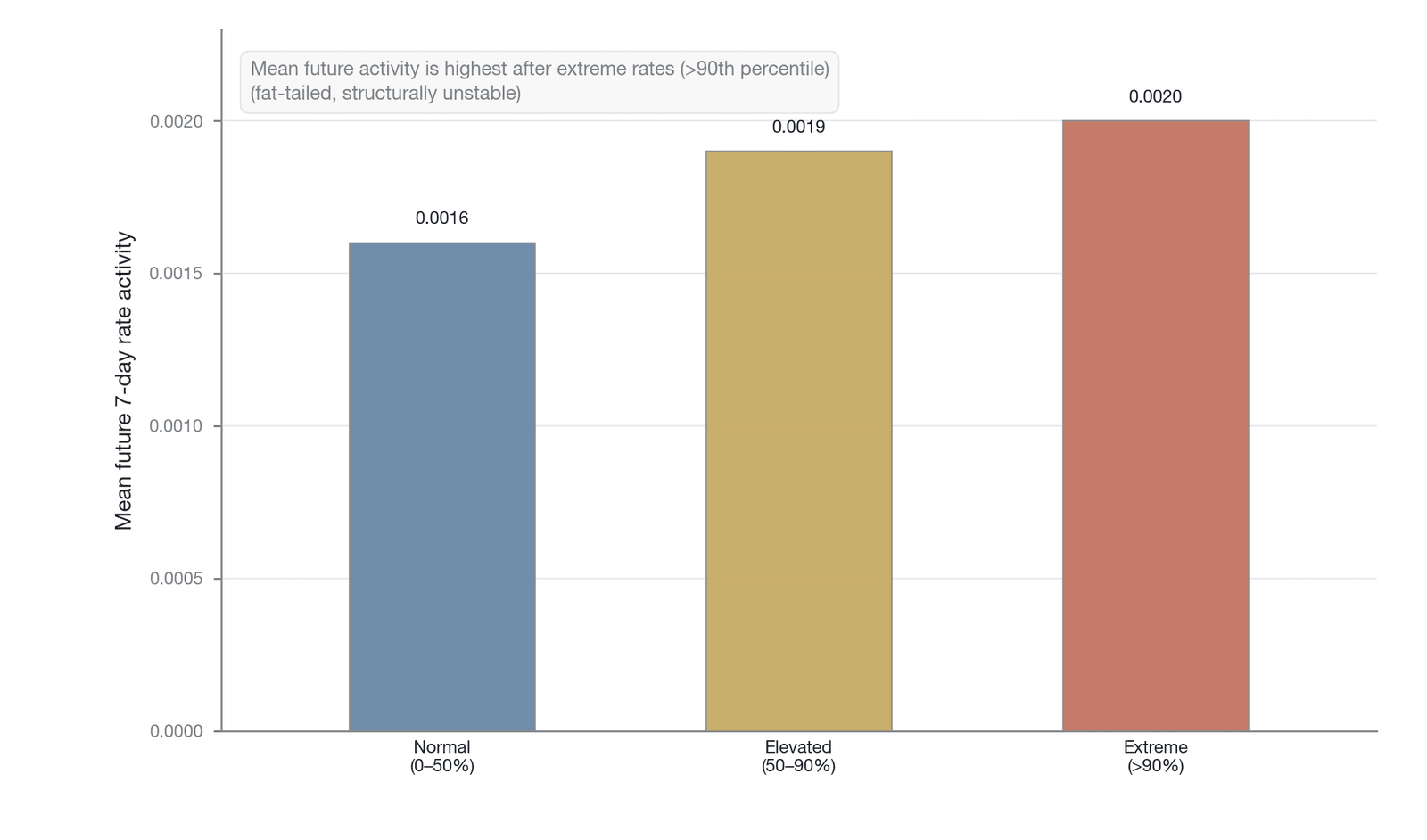
Figure 10-26. The distribution of funding rate activity over the next 7 days following an extreme rate state (computed by the author from the Hyperliquid API; descriptive; sample period September 2025 to March 2026, single exchange) [33]
Figure 10-26 clearly shows that when the market is in an "extreme rate" state (above the 90th percentile of the historical absolute-value distribution), the rate activity over the subsequent 7 days (i.e., the sum of absolute rate changes) exhibits a pronounced fat-tailed distribution, with a mean significantly higher than in the normal and elevated rate states. This means that an extreme rate not only foreshadows future high volatility but also foreshadows a structural instability. Once the rate enters the extreme range, the market rarely calms down quickly; instead, it undergoes a sustained period of turmoil until leverage is thoroughly cleared and a new equilibrium is established.
10.8.3 The cross-asset funding rate surface
Extending the view from a single asset to the entire market, the funding rate constructs a multidimensional cross-asset surface. Strictly speaking, perpetual futures have no "term structure" in the traditional sense (because there is no expiry date), but we can construct an analogous information surface along two dimensions: the cross-asset dimension and the cross-exchange dimension. This surface is one of the high-frequency indicators for characterizing the cross-asset distribution of speculative heat.
Along the cross-asset dimension, the rates of BTC, ETH, SOL, and various altcoins reflect the intensity of directional preference for different assets. Altcoin rates are usually far higher than BTC's, reflecting stronger speculative preference and lower arbitrage efficiency. Along the cross-exchange dimension, the rate differences for the same asset across platforms such as Binance, Bybit, Hyperliquid, and dYdX reflect differences in each platform's user composition and liquidity structure. Boros Finance's data show that the rate difference between Binance and Hyperliquid can reach a significant level, providing considerable return space for cross-exchange arbitrage (the specific return ranges are given in Section 10.4.2 and Figure 10-10) [22].
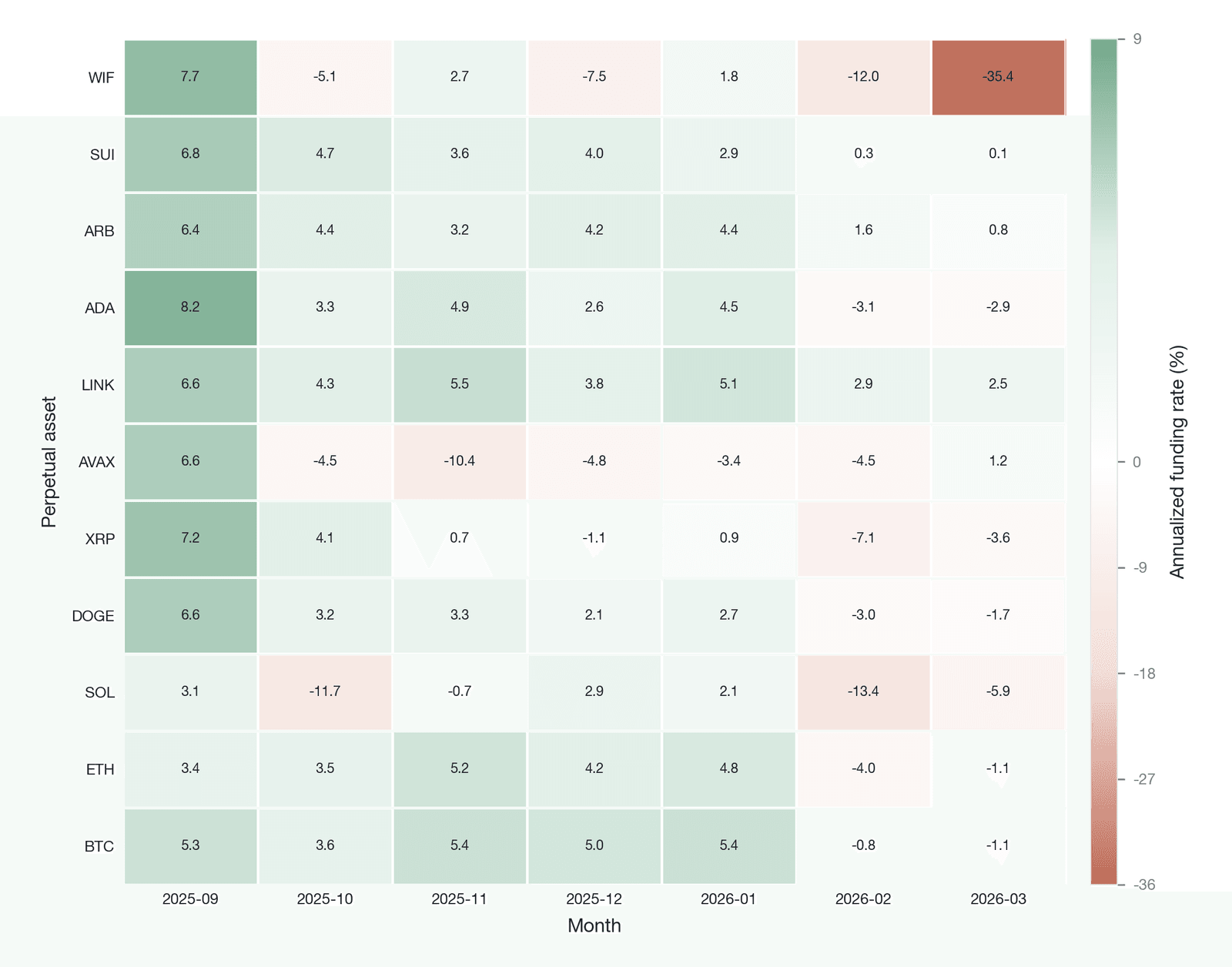
Figure 10-27. A monthly heatmap of cross-asset funding rates (all values are measured funding rates for Binance USDT perpetuals, annualized from each asset's mean per-period rate for the month; sample period September 2025 to March 2026, as of June 30, 2026)
The cross-asset heatmap in Figure 10-27 reveals several patterns. The cornerstone assets exhibit high stability: the rates of BTC and ETH are relatively stable, staying in a mild positive range in most months (about 3%–5% annualized) and turning slightly negative only in early 2026, with a volatility clearly smaller than that of altcoins, reflecting their status as market benchmarks and the ample arbitrage liquidity in their derivatives markets. Long-tail assets fluctuate more widely: relative to BTC, long-tail assets (such as WIF, SOL, and OP) exhibit extreme rate fluctuations. For example, according to measured Binance data, WIF's annualized rate plunged to about −35.4% in March 2026 and SOL's fell to about −13.4% in February 2026, indicating that these assets were undergoing intense shorting pressure or a liquidity crisis. Sector rotation is the final dimension: by watching which assets carry high rates from month to month, one can track the movement of speculative capital. In September 2025, most altcoin rates rose collectively (ADA and WIF reached about 8.2% and 7.7%, respectively), but by early 2026 most turned negative (for example, AVAX fell from about 6.6% in September to about −10.4% in November), while LINK maintained a stable positive rate throughout the observation period. When the assets of a sector collectively exhibit high positive rates, this is often a clear signal that the sector is overheated.
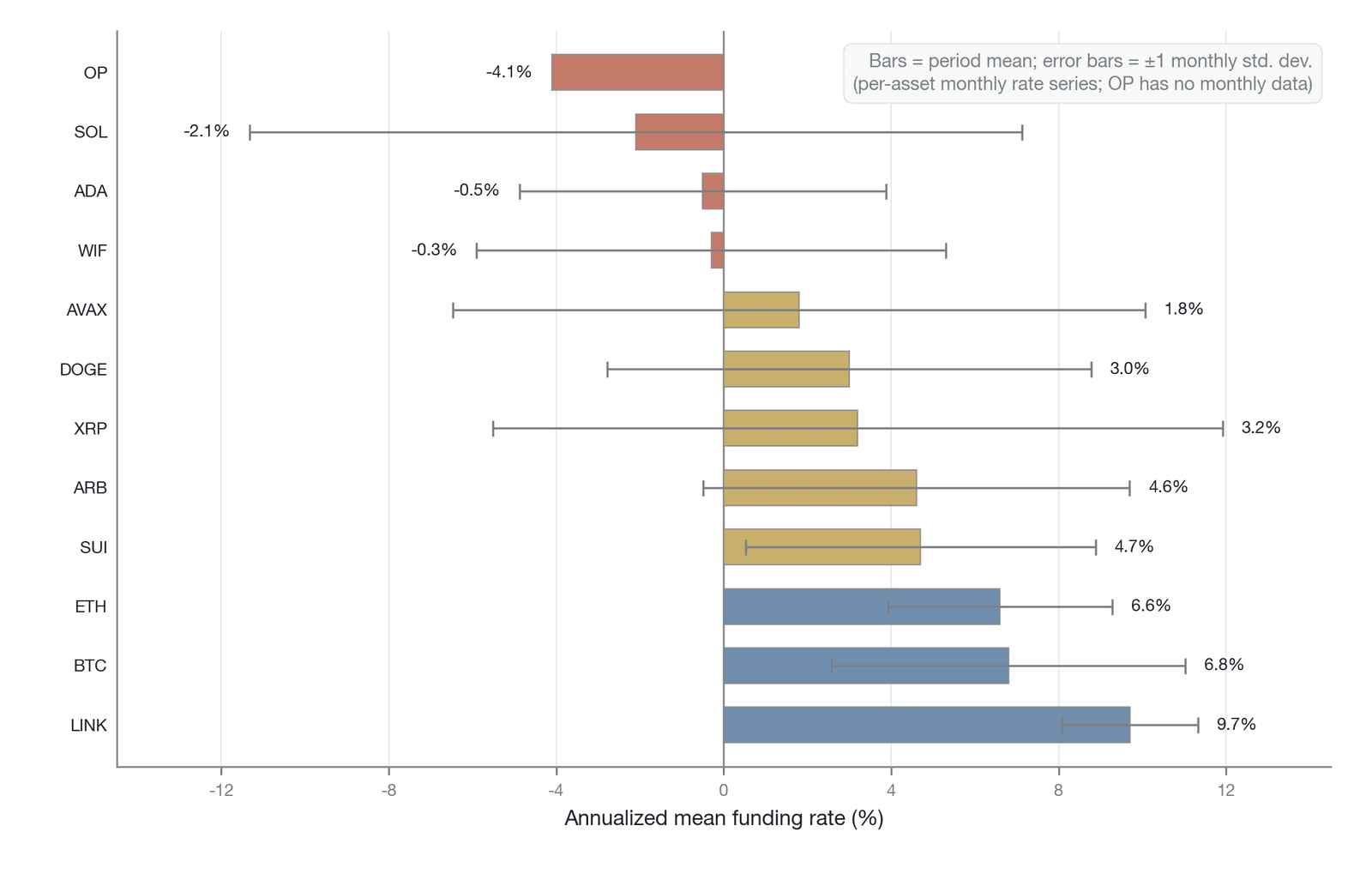
Figure 10-28. A comparison of cross-asset annualized average funding rates with standard-deviation ranges (computed by the author from the Hyperliquid API; descriptive; sample period September 2025 to March 2026, single exchange) [33]
Figure 10-28 further shows the overall rate characteristics of different assets over the observation period. LINK (9.7%) and BTC (6.8%) maintained relatively high positive rates, while OP (−4.1%), SOL (−2.1%), and ADA (−0.5%) exhibited a structural negative rate. Such a long-term structural difference often stems from microstructural friction in a particular asset's spot lending market, or from the specific role the asset plays in hedging strategies (such as cash-and-carry arbitrage or staking-mining hedges).
In addition, the rate correlation between BTC and ETH constitutes an independent macro state variable. When their rates are highly positively correlated, the market is being driven by a unified macro force (such as Federal Reserve policy expectations or ETF inflows) and systemic risk is highly concentrated; when the correlation falls or even turns negative, capital is being allocated differentially based on asset-specific narratives (such as an Ethereum upgrade or a Bitcoin halving), and the market is in a phase of structural divergence. For a trader holding a multi-asset portfolio, a sudden change in rate correlation is a key signal for adjusting the hedge ratio.
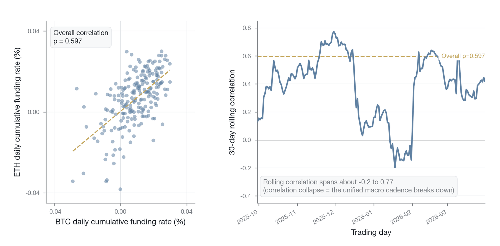
Figure 10-29. A scatter plot of daily BTC and ETH funding rates and their 30-day rolling correlation (Data source: measured daily cumulative funding rates for BTC and ETH perpetuals on Binance, September 2025 to March 2026; as of June 30, 2026)
As Figure 10-29 shows, although BTC and ETH maintained an overall positive correlation of about 0.597 over the sample period, their 30-day rolling correlation coefficient exhibited pronounced time variation (ranging from about −0.20 to 0.77). A collapse in correlation often carries far-reaching systemic implications. When the rates of BTC and ETH diverge, it usually means that the unified pace of macro capital has been broken and the market has entered a phase of structural divergence based on asset-specific narratives (such as expectations of an Ethereum upgrade or Bitcoin ETF inflows). Conversely, when the correlation rises sharply to a high level, it often means the market is in a state of systemic risk-on or risk-off, with all assets driven by the same macro force.
Two methodological qualifications are in order. First, a correlation collapse may partly reflect a macro-level flight-to-quality effect (BTC receiving safe-haven inflows on the "digital gold" narrative while ETH comes under pressure from DeFi deleveraging), rather than pure crypto-native narrative rotation. A formal attribution analysis should introduce macro control variables (such as the U.S. Dollar Index (DXY) and the global risk-appetite gauge VIX) to distinguish the relative contributions of macro transmission and crypto-native factors. Second, the BTC-ETH bivariate analysis can naturally be extended to a principal component analysis (PCA) of the full-sample (10+ assets) rate correlation matrix. If the variance explained by the first principal component surges from about 40% in normal periods to more than 80% in a crisis, it would confirm the hypothesis that "rates collapse into a single systemic factor in a crisis." This constitutes a natural extension for future research.
10.8.4 Comparison with traditional sentiment indicators
In both traditional financial markets and the crypto market, there are many indicators for measuring market sentiment and state. The funding rate, however, has advantages over survey- or text-based sentiment indicators along two dimensions—directness and economic consequence—the core reason being "the price paid in real money."
Most traditional sentiment indicators are indirect, inferential, or soft indicators based on questionnaires and text analysis. The funding rate, by contrast, is a cash flow that market participants must actually pay to maintain their directional exposure. Table 10-8 systematically compares the funding rate with the main traditional sentiment indicators:
| Indicator | Data basis | Update frequency | What it measures | Directness for the perpetual futures market |
|---|---|---|---|---|
| Funding rate | Long-short imbalance in perpetual futures | Every 1–8 hours | Leverage cost = a direct measure of risk | Extremely direct: generated by the market itself, with real economic consequences |
| VIX | Implied volatility of S&P 500 options | Continuous | Expected volatility over the next 30 days | Indirect: measures the traditional market, not directly corresponding to crypto |
| Put/call ratio | Options volume | Daily | Bearish vs. bullish sentiment | Indirect: the crypto options market is far smaller than the perpetual futures market |
| Fear and Greed Index | Multi-factor composite | Daily | A composite measure of fear/greed | Indirect: factor weights are subjective and not reproducible |
| Social-media sentiment | Text sentiment analysis | Real-time | The direction of public sentiment | Indirect: noisy and easily manipulated |
| Open interest | Derivatives position size | Continuous | Total leverage accumulation | Relatively direct: but contains no directional information |
Table 10-8. A multidimensional comparison of the funding rate with traditional sentiment indicators (Data source: compiled by the author)
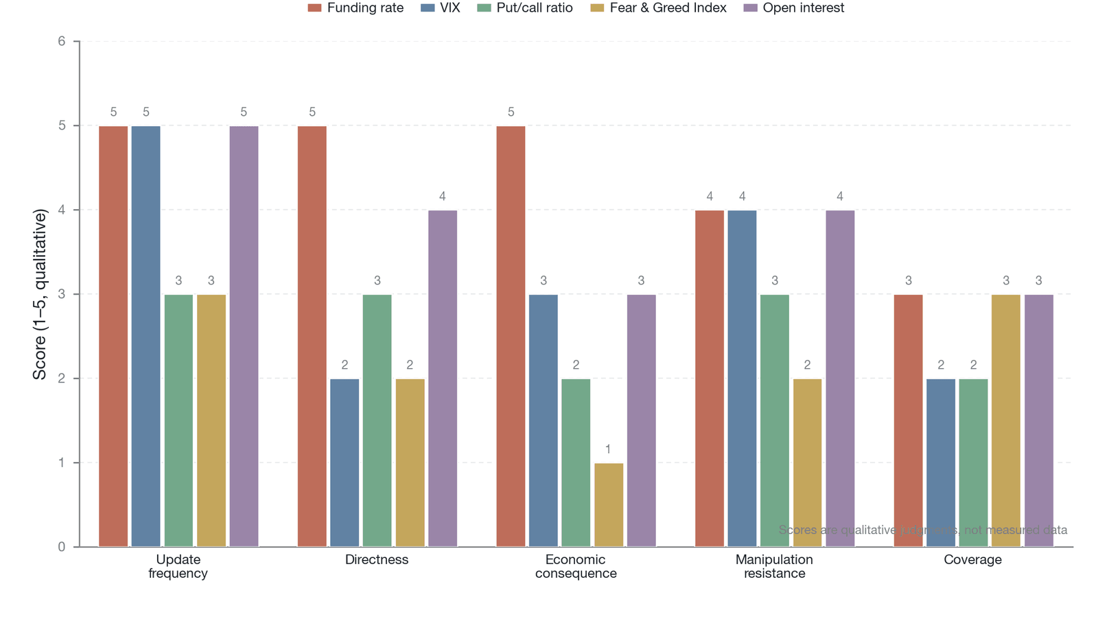
Figure 10-30. A multidimensional comparison of the funding rate with traditional sentiment indicators (subjective/qualitative 1–5 scoring, assessed by the author, not quantitative measurement; the dimensions correspond to Table 10-8 in the main text, the figure shows a selection of five representative indicators, and the cross-comparison reflects the author's judgment)
The predictive value of the rate stems from its directness: it is not a sentiment indicator derived indirectly through an intermediate model but a price signal, with real economic consequences, generated by the perpetual futures market itself every 1–8 hours. Traders actually pay or receive the rate each period, which gives the rate higher credibility than survey- or model-based indicators.
As the comparative analysis in Figure 10-30 shows, the funding rate demonstrates unique advantages along several dimensions. On directness and economic consequence, an extreme value of the Fear and Greed Index does not directly bankrupt any market participant, but an extreme funding rate does: a high rate genuinely erodes margin and forces traders to close positions, thereby directly triggering a chain price reaction. It not only measures risk; it is itself a catalyst of risk. On update frequency, most traditional indicators are daily, whereas the funding rate is updated continuously or at high frequency (such as hourly or every 8 hours), capturing instantaneous shifts in market sentiment at extremely fine granularity. On manipulation resistance, social-media sentiment or questionnaires are easily manipulated by bots or coordinated behavior, whereas to manipulate the funding rate, a manipulator must build a real, large one-sided position in the derivatives market and bear the enormous price risk and friction cost that entails. On directional clarity, unlike total open interest, which can show only the scale of leverage, the sign of the funding rate directly gives the direction of the leverage tilt.
The funding rate is not a description of market sentiment but the pricing of market sentiment. This distinction carries important methodological significance: the Fear and Greed Index or social-media sentiment analysis belongs to the category of "observation," and a researcher can obtain and interpret these signals at no cost; the funding rate belongs to the category of "pricing," and every position holder is paying for its directional view with real cash flow. This economic constraint makes the noise in the rate signal inherently lower than that in cost-free observational indicators, because traders holding positions in the wrong direction are continuously drained by the rate until they exit.
10.8.5 Empirical evidence and limitations of predictive power
Based on the analysis above, the funding rate as a state variable exhibits, at the descriptive level, statistical associations consistent with systemic fragility, volatility bursts, and cross-asset rotation. Existing academic research also supports this judgment. Inan (2025) shows that the funding rate of perpetual futures has significant out-of-sample predictability, indicating that the rate encodes forward-looking information about the state of the Bitcoin market [34]. Presto Research (2024) finds a statistically significant but weak positive correlation between rate changes and contemporaneous price changes (R² of about 12.5%), but near-zero out-of-sample predictive power for the next-period price change of a single asset; that study did not specifically test extreme rates or price reversals [35].
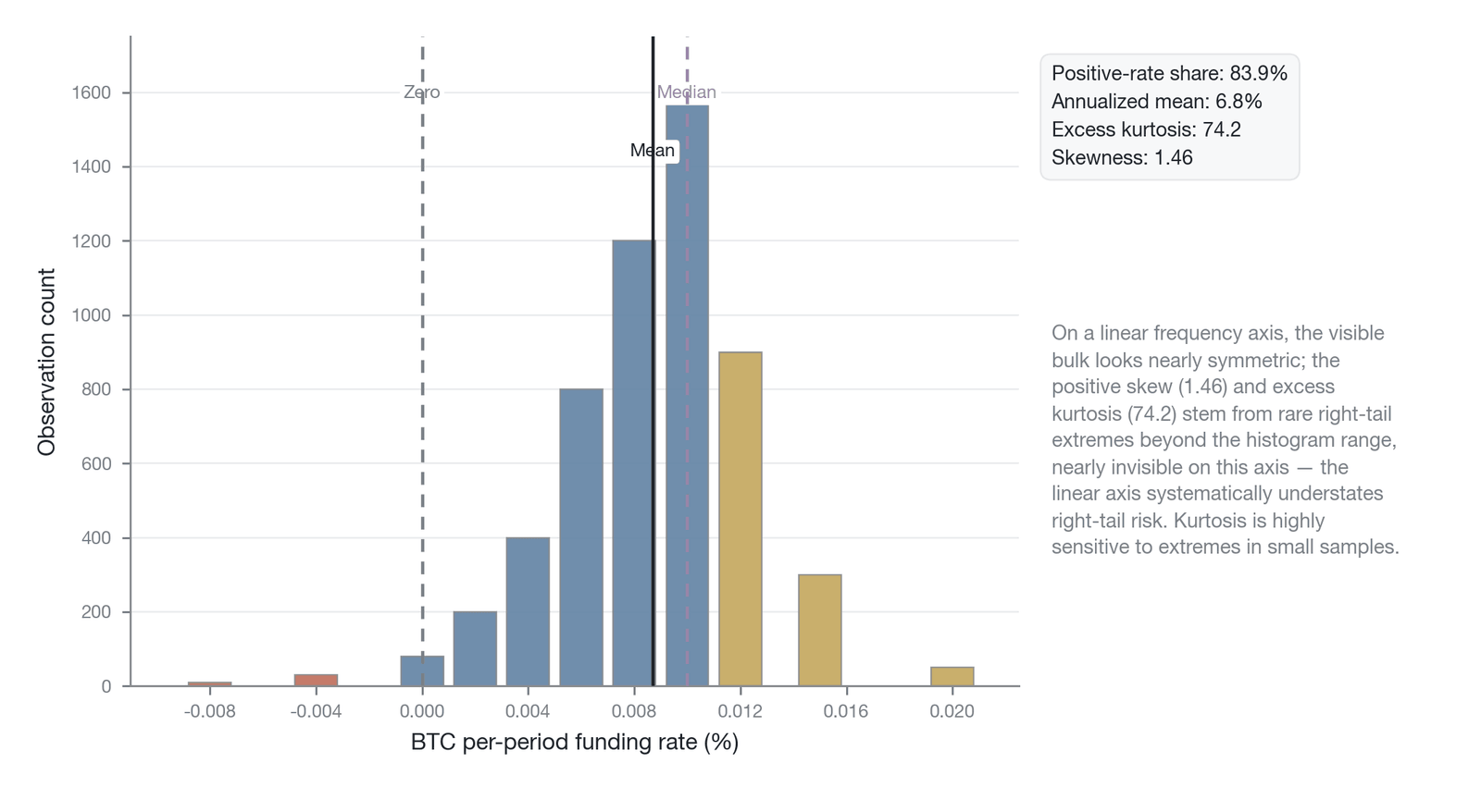
Figure 10-31. The asymmetry and long-tail characteristics of the BTC funding rate distribution (the distribution statistics—skewness, excess kurtosis, positive-rate share, annualized mean, etc.—are computed by the author from the Hyperliquid API; descriptive and sensitive to extreme values in small samples [33]; the predictability R² ≈ 12.5% is cited from [35] and the out-of-sample predictability from [34])
Figure 10-31 shows the empirical distribution of the BTC funding rate. Its distribution exhibits extreme positive skew (skewness = 1.46) and very high kurtosis (excess kurtosis = 74.2, i.e., the deviation relative to the normal-distribution kurtosis of 3; note that this estimate is highly sensitive to extreme observations in small samples). The positive-rate share is as high as 83.9% and the annualized mean is about 6.8%, confirming the long-standing "structural long bias" of the cryptocurrency market. This extreme non-normal distribution means that traditional finance models based on the normality assumption will fail severely when handling the funding rate, and the rate's tail risk (especially the right tail) far exceeds theoretical expectations.
The empirical evidence presented in this section is descriptive rather than a formal inferential test. The conditional relationship between the rate level and future volatility shown in Figures 10-24 through 10-26, although consistent with economic intuition, has not been rigorously validated through multivariate regression controlling for other predictor variables (such as realized volatility and the rate of change of open interest) or through Granger causality tests. In addition, the Hyperliquid data [33] used in this chapter have the limitations of a short sample period (September 2025 to March 2026, about six months) and a single-exchange source; differences in user composition and liquidity characteristics across exchanges may cause heterogeneity in rate dynamics, and conclusions drawn from a single platform are not necessarily universally applicable across platforms. Elevating the descriptive findings to formal predictive regressions and out-of-sample tests is a priority direction for future research. Specifically, a standard predictive regression specification can be written as:
where is the realized volatility over the next 7 days, is the absolute value of the current rate, is the current realized volatility (controlling for the volatility-clustering effect), and is the rate of change of open interest. Because the overlapping 7-day window of introduces moving-average autocorrelation, a formal inferential test should use Newey-West heteroskedasticity- and autocorrelation-consistent standard errors, with a lag truncation parameter no less than the window length (i.e., 7 periods). If remains statistically significantly positive after controlling for and , the incremental predictive power of the rate level for future volatility can be formally confirmed. The current evidence supports this direction at the level of the conditional distribution, but rigorous statistical inference is left for subsequent research on a longer sample period and multi-exchange data.
At the methodological level, two technical issues also warrant attention. The first is collinearity: and may be highly collinear, since in a high-volatility environment the rate itself tends to be more extreme, which may destabilize the estimate of . Mitigations include orthogonalization or principal-component methods, or using a HAR-RV-style multi-scale benchmark model (introducing daily/weekly/monthly realized-volatility components) and testing as an incremental predictor to gauge its marginal contribution after controlling for known volatility persistence. The second is the characterization of the evidence: the nature of the current evidence should be labeled more explicitly. The conditional-distribution comparisons shown in Figures 10-24 through 10-28 are descriptive analysis, and moving from descriptive findings to a formal predictive-causal claim requires completing out-of-sample tests with multivariate controls (such as rolling-window out-of-sample R²). These two methodological improvements are the necessary steps for turning the chapter's descriptive findings into a rigorous predictive model.
Using the funding rate as a predictor, however, also has inherent limitations that must be treated with care.
On timeliness, an extreme funding rate can signal with high confidence that the system is fragile, but it cannot pinpoint the timing of a collapse. A market can persist in an irrationally high-rate state for weeks or even months (as in the first quarter of 2021 or the early-2024 bull phase), and shorting too early on the basis of a high rate may lead to severe paper losses. The rate's predictive power lies mainly in the volatility dimension: it can indicate that the probability of a volatility increase is rising, but it cannot pinpoint direction or timing. This is similar in nature to the predictive power of VIX and is an inherent limitation of the funding rate as a state variable. Structural shifts are a second confounding factor. As noted in Section 10.2, the rate contains a financing cost layer, and when the macro risk-free rate changes sharply (such as during a Federal Reserve hiking cycle) or when structural friction appears in the spot lending market, the center of the rate shifts. Without using the three-layer decomposition model to strip away these structural factors, looking only at the absolute rate level may produce false overheating or over-cooling signals. In addition, the trend of rate financialization is lowering the rate's signal-to-noise ratio as a sentiment indicator: with the rise of systematic arbitrage entities such as Ethena, extreme rates are flattened faster, and when large amounts of capital systematically short perpetual futures to earn a positive rate, their collective behavior itself becomes a force depressing the rate, forming a new reflexive loop in which more rate changes reflect only the entry and exit of arbitrage capital rather than genuine speculative sentiment. This structural impact of rate financialization and its dilution of the state variable hypothesis are developed in Section 10.8.6.
In sum, the funding rate is a powerful state variable that requires careful interpretation. It is not a simple "overbought/oversold" oscillator but a comprehensive macro indicator reflecting the market's leverage structure, liquidity condition, and arbitrage-game equilibrium. Using it correctly requires combining the three-layer decomposition model to strip away structural factors, the volatility dimension to judge uncertainty, and the cross-asset surface to locate the risk distribution. Only in this way can the rate be refined from a crude directional signal into a precise diagnostic tool for the market state.
10.8.6 Rate financialization: Ethena and the funding rate swap market
The analytical framework of the funding rate as a state variable is facing a structural challenge: the funding rate itself is evolving from a passive holding cost into a financial asset that can be independently traded, hedged, and structured. This transformation, represented by the Ethena protocol and Boros Finance's funding rate swap products, marks the arrival of the era of "rate financialization."
Ethena's USDe stablecoin is the most systemically significant instance of rate financialization. USDe's core mechanism is to hold spot ETH (or BTC) and establish an equal-size short position in the perpetual futures market, thereby systematically collecting the positive funding rate in a market-neutral manner. As of early 2026, USDe's size has reached billions of dollars, making Ethena an important structural short seller in the perpetual futures market (accounting for several percent of ETH perpetual open interest, per reports from outlets such as The Block). Ethena's scale effect has a dual impact on the rate market. On the supply side, billions of dollars in persistent short positions inject stable sell-side liquidity into a positive-rate environment, accelerating the rate's return to equilibrium in normal markets and objectively strengthening the anchoring mechanism. On the crisis side, however, when the rate suddenly turns negative (as during the panic selling triggered by the DeepSeek event in late January 2025), Ethena's enormous short positions face reverse rate-outlay pressure. At that point, Ethena not only cannot collect income but becomes a net payer of the rate, and its forced position-reduction may further intensify market volatility.
More systematically, the risks Ethena faces can be analyzed along three dimensions. On the economic-risk contagion path: a persistently negative rate → USDe yield turns negative → large-scale redemptions by holders → Ethena is forced to close short positions (executing large buys in the contract market) → an upward price shock is produced → if the redemption pressure causes USDe to depeg, its role as widely used collateral in DeFi lending protocols will amplify cross-protocol contagion. On the operational-risk dimension: Ethena holds billions of dollars in short positions on centralized exchanges, facing exchange custody risk (the roughly $1.5 billion hack of Bybit in February 2025 is a real-world warning of this kind of risk), account-freeze risk, and execution-slippage risk when rebalancing large positions across exchanges. On the regulatory-risk dimension: USDe's yield mechanism may be characterized by the SEC as an unregistered investment contract (the Howey test)—users deposit funds and expect returns from an actively managed strategy run by the team, which fits the characteristics of an investment contract closely; in addition, the stablecoin classification and reserve requirements under the EU's Markets in Crypto-Assets (MiCA) framework may also constrain USDe's compliance.
Funding rate swap products such as those of Boros Finance push rate financialization from another dimension. A funding rate swap allows a trader to convert floating funding-rate exposure into a fixed yield (or vice versa), essentially creating a derivatives market with the funding rate as the underlying asset—a "derivative of a derivative." Such products enable institutional investors to express a view on rate direction or volatility purely, without holding any perpetual futures position.
The core impact of rate financialization on the state variable hypothesis is a decline in the signal-to-noise ratio. As a growing share of rate changes reflect the capital inflows and outflows of arbitrage entities such as Ethena rather than genuine shifts in speculative sentiment, the rate's signal value as a "market thermometer" is systematically diluted. Quantifying this dilution effect (for example, by decomposing rate changes into a component from systematic arbitrage capital and a component from directional speculation) is an important topic for future research. Chapter 18 will further analyze the long-term impact of Ethena's scale expansion on the market microstructure from a systemic-risk perspective.
10.9 Chapter summary
This chapter has conducted a systematic game-theoretic analysis of the core mechanism of perpetual futures—the funding rate—from micro mechanism to macro state. The funding rate is not a simple interest-payment formula but an automatic regulator arising from the interaction of multiple layers of games in the crypto derivatives market. The chapter's analysis is organized around five nested theoretical frameworks.
The three-layer decomposition model deconstructs the apparently single funding rate into a financing cost layer (a slowly varying institutional benchmark, about 10.95% annualized), a sentiment premium layer (the high-frequency directional preference of the market), and an institutional friction layer (the stable-band effect created by the clamp function; BitMEX research shows the rate is locked exactly at 0.01% for 78.19% of the time [8]). This framework shows that the rate is in fact a hybrid product of the macro interest rate, market speculative preference, and microstructural contract design, and that only by separating the three layers can the meaning of the rate signal be accurately diagnosed.
Building on this, the anchoring strength spectrum reveals the nonlinear character of the funding rate's effectiveness. Anchoring strength is a monotonically increasing function of the intensity of arbitrage activity, and arbitrage weakens systemically in extreme markets because six conditions—capital constraints, counterparty risk, liquidity drought, execution risk, liquidation risk, and cross-asset margin contagion—deteriorate simultaneously. The resulting anchoring paradox—that anchoring strength falls to its lowest precisely when the market most needs anchoring—is validated in events such as the March 12, 2020 episode when the BTC perpetual price fell hundreds of dollars below spot [5] and the October 10, 2025 episode with a visible 24-hour liquidation notional of about $19 billion [17].
The analytical framework of anchoring strength extends further into the three-layer game model, which abstracts the dynamic evolution of the funding rate into three nested games: the innermost anchoring game (the war of attrition and reflexive loop between longs and shorts over the basis), the middle convergence game (cash-and-carry arbitrageurs driving price convergence and cross-exchange arbitrageurs driving rate convergence; the annualized return ranges of cross-exchange arbitrage are given in Section 10.4.2 [22]), and the outermost strategic game (the rules attack and defense between exchanges and attackers). The balance of forces among the three layers determines the markedly different dynamics the rate exhibits in the normal, stress, and crisis market states.
When the game equilibrium is broken, the rate polarization positive feedback mechanism is set in motion. The condition for the flip from negative to positive feedback is that the directional profit exceeds the rate cost, while the disposition effect, confirmation bias, and herding jointly drive holders' refusal to close. Polarization terminates in only one of two ways: mild mean reversion or a liquidation cascade. In the PIPPIN case, shorts' rate outlay alone reached −19.77% of notional principal within 24 hours, illustrating the effect of positive feedback amplified by high-frequency settlement. Rate polarization thereby becomes a directly observable signal that the leverage cycle is approaching its critical point, which leads to the chapter's fifth framework—the funding rate as state variable hypothesis—elevating the rate from a passive output variable to an active macro state variable.
Figure 10-32 integrates the three information dimensions of the rate (level, volatility, and the cross-asset surface) with their corresponding analytical outputs into a systematic analytical framework.
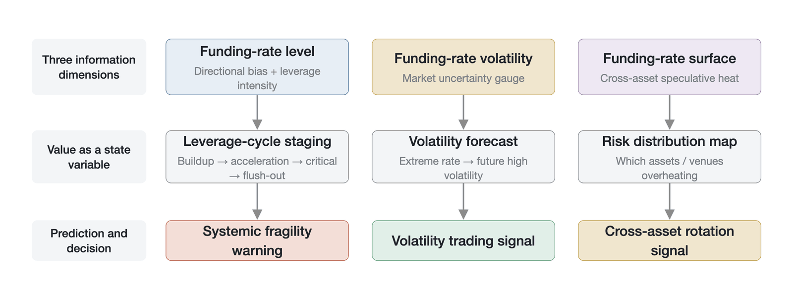
Figure 10-32. The analytical framework and application path of the funding rate as a state variable (a conceptual illustration based on the analytical framework, not empirical data)
As Figure 10-32 shows, the rate's level, volatility, and cross-asset surface together form a multidimensional analytical matrix capable of identifying the phase of the leverage cycle, predicting future volatility bursts, and mapping the risk distribution of the entire market. Compared with indirect indicators such as VIX, the funding rate can reflect the market's leverage-structure state at higher frequency and with lower latency. The spot price reflects the market's instantaneous supply and demand, while the funding rate reveals the market's leverage structure: the rate continuously prices the positions of longs and shorts through actual cash-flow transfers, and the flow of arbitrage capital delineates the effectiveness boundary of the anchoring mechanism. At the same time, the trend of rate financialization is creating a new game dimension: when the rate itself becomes a tradable asset, the game around it will grow more complex still.
The funding rate does not exist in isolation. It is closely linked to the accumulation of leverage, the triggering of the liquidation mechanism, and the depth of liquidity pools. The chapter's analysis points to a core conclusion: the boundary of the funding rate's anchoring efficacy is precisely the starting point at which leverage and liquidation risk begin to dominate the market. When the rate loses its anchoring force in a crisis state, what takes over the market is no longer the game of long-short willingness but the forced execution of the liquidation mechanism. The next chapter starts from this breaking point of rate failure and enters the extreme-risk domain of the liquidation cascade, analyzing how the forced-liquidation mechanism operates and fails when the price breaches the maintenance-margin floor. The funding rate determines the cost of leverage, while the liquidation mechanism determines the survival of leveraged positions.
References
[1] James, N. (2021). Changes to the extreme and erratic behaviour of cryptocurrencies during COVID-19. Physica A: Statistical Mechanics and its Applications, 565, 125462. https://pmc.ncbi.nlm.nih.gov/articles/PMC7687370/ https://doi.org/10.1016/j.physa.2020.125581
[2] Godbole, O. (2020, March 13). Bitcoin price briefly dips to 12-month low in overnight trading. CoinDesk. https://www.coindesk.com/markets/2020/03/13/bitcoin-price-briefly-dips-to-12-month-low-in-overnight-trading
[3] CoinDesk. (2020, March 12). Bitcoin's crash triggers over \$700M in liquidations on BitMEX. https://www.coindesk.com/markets/2020/03/12/bitcoins-crash-triggers-over-700m-in-liquidations-on-bitmex
[4] CryptoSlate. (2020). BitMEX freezes as XBTUSD crashes 10% below Bitcoin spot price. https://cryptoslate.com/bitmex-freezes-as-xbtusd-crashes-10-below-bitcoin-spot-price/
[5] Multicoin Capital. (2020, March 17). March 12: The day crypto market structure broke (Part 1). https://multicoin.capital/2020/03/17/march-12-the-day-crypto-market-structure-broke/
[6] Alexander, C., Choi, J., Park, H., & Sohn, S. (2020). BitMEX bitcoin derivatives: Price discovery, informational efficiency, and hedging effectiveness. Journal of Futures Markets, 40(1), 23–100. https://onlinelibrary.wiley.com/doi/abs/10.1002/fut.22050 https://doi.org/10.1002/fut.22050
[7] MilkRoad. (n.d.). Perpetual contracts: Definitions & FAQ for funding rates. https://milkroad.com/funding/perpetual-contracts/
[8] BitMEX Research. (2025). Funding rates structure: Floor & ceiling explained — Q3 2025 derivatives report. https://www.bitmex.com/blog/2025q3-derivatives-report [Industry report, not peer-reviewed]
[9] Palepu, A. (2020, June 23). Funding rates: Under the hood. Medium / DerivaDEX. https://medium.com/derivadex/funding-rates-under-the-hood-352e6be83ab
[10] Binance Support. (2025). Important updates on funding rate settlement frequency. https://www.binance.com/en/support/announcement/detail/6d707b1f7ae34f419621b4c807464ab1
[11] Hyperliquid. (n.d.). Funding. Hyperliquid Documentation. https://hyperliquid.gitbook.io/hyperliquid-docs/trading/funding
[12] Schmeling, M., Schrimpf, A., & Todorov, K. (2023). Crypto carry (BIS Working Paper No. 1087). Bank for International Settlements. https://www.bis.org/publ/work1087.htm
[13] Bloomberg. (2026, January 21). Wall Street pulls back from a money-spinning Bitcoin trade.
[14] Ackerer, D., Hugonnier, J., & Jermann, U. (2025). Perpetual futures pricing. Mathematical Finance. https://doi.org/10.1111/mafi.70018
[15] Gabaix, X., & Maggiori, M. (2015). International liquidity and exchange rate dynamics. Quarterly Journal of Economics, 130(3), 1369–1420. https://doi.org/10.1093/qje/qjv016
[16] Brunnermeier, M. K., & Pedersen, L. H. (2009). Market liquidity and funding liquidity. Review of Financial Studies, 22(6), 2201–2238. https://doi.org/10.1093/rfs/hhn098
[17] CoinShares. (2025, October 20). Billions in crypto liquidations: Inside October's \$19B crash.
[18] Shleifer, A., & Vishny, R. W. (1997). The limits of arbitrage. Journal of Finance, 52(1), 35–55. https://doi.org/10.1111/j.1540-6261.1997.tb03807.x
[19] Scheinkman, J. A., & Xiong, W. (2003). Overconfidence and speculative bubbles. Journal of Political Economy, 111(6), 1183–1220. https://doi.org/10.1086/378531
[20] Collins, T. (2025). The future of Bitcoin: Market maturity, strategic reserves, and the paradox of institutional accumulation. SSRN. https://papers.ssrn.com/sol3/papers.cfm?abstract_id=5788582 https://doi.org/10.2139/ssrn.5788582
[21] De Long, J. B., Shleifer, A., Summers, L. H., & Waldmann, R. J. (1990). Noise trader risk in financial markets. Journal of Political Economy, 98(4), 703–738. https://doi.org/10.1086/261703
[22] Pendle Team. (2025, December 19). Cross-exchange funding rate arbitrage: A fixed-yield strategy through Boros. Medium / Boros Finance. https://medium.com/boros-fi/cross-exchange-funding-rate-arbitrage-a-fixed-yield-strategy-through-boros-c9e828b61215 [Industry report, not peer-reviewed]
[23] Baumgartner, T., & Guettler, A. (2022). Trust in a trustless network: The case of the Bitcoin flash crash on May 19, 2021. EUROFIDAI-ESSEC Paris December Finance Meeting. https://papers.ssrn.com/sol3/papers.cfm?abstract_id=4260876 https://doi.org/10.2139/ssrn.4260876
[24] Gromb, D., & Vayanos, D. (2002). Equilibrium and welfare in markets with financially constrained arbitrageurs. Journal of Financial Economics, 66(2–3), 361–407. https://doi.org/10.1016/S0304-405X(02)00228-3
[25] CoinDesk. (2021). Bitcoin drops below \$31K before rebounding; \$8B in liquidations triggered.
[26] Kahneman, D. (2011). Thinking, Fast and Slow. Farrar, Straus and Giroux.
[27] Binance Square. (2025). The reasons behind Alpaca's pre-delisting short squeeze.
[28] Skwarek, M. (2025). Why do investors behave irrationally in the cryptocurrency and emerging stock markets? SAGE Open, 15(3). https://doi.org/10.1177/21582440251361212
[29] Banerjee, A. V. (1992). A simple model of herd behavior. Quarterly Journal of Economics, 107(3), 797–817. https://doi.org/10.2307/2118364
[30] Delfabbro, P., King, D. L., & Williams, J. (2021). The psychology of cryptocurrency trading: Risk and protective factors. Journal of Behavioral Addictions, 10(2), 201–207. https://doi.org/10.1556/2006.2021.00037
[31] Minsky, H. P. (1992). The financial instability hypothesis (Working Paper No. 74). The Jerome Levy Economics Institute of Bard College. https://www.levyinstitute.org/pubs/wp74.pdf
[32] U.S. Department of Justice. (2023, January 10). Avraham Eisenberg charged in connection with manipulation of Mango Markets decentralized cryptocurrency exchange. https://www.justice.gov/usao-sdny/pr/avraham-eisenberg-charged-connection-manipulation-mango-markets
[33] Hyperliquid. (2026). Hyperliquid API documentation: Funding rate history. https://hyperliquid.xyz/
[34] Inan, E. (2025). Predictability of funding rates (SSRN Working Paper No. 5576424). https://doi.org/10.2139/ssrn.5576424
[35] Presto Research. (2024, August 2). Can funding rate predict price change? https://www.prestolabs.io/research/can-funding-rate-predict-price-change